In this tutorial, you’ll get a thorough introduction to the k-Nearest Neighbors (kNN) algorithm in Python. The kNN algorithm is one of the most famous machine learning algorithms and an absolute must-have in your machine learning toolbox. Python is the go-to programming language for machine learning, so what better way to discover kNN than with Python’s famous packages NumPy and scikit-learn!
Below, you’ll explore the kNN algorithm both in theory and in practice. While many tutorials skip the theoretical part and focus only on the use of libraries, you don’t want to be dependent on automated packages for your machine learning. It’s important to learn about the mechanics of machine learning algorithms to understand their potential and limitations.
At the same time, it’s essential to understand how to use an algorithm in practice. With that in mind, in the second part of this tutorial, you’ll focus on the use of kNN in the Python library scikit-learn, with advanced tips for pushing performance to the max.
In this tutorial, you’ll learn how to:
- Explain the kNN algorithm both intuitively and mathematically
- Implement kNN in Python from scratch using NumPy
- Use kNN in Python with scikit-learn
- Tune hyperparameters of kNN using
GridSearchCV - Add bagging to kNN for better performance
Free Bonus: Click here to get access to a free NumPy Resources Guide that points you to the best tutorials, videos, and books for improving your NumPy skills.
Basics of Machine Learning
To get you on board, it’s worth taking a step back and doing a quick survey of machine learning in general. In this section, you’ll get an introduction to the fundamental idea behind machine learning, and you’ll see how the kNN algorithm relates to other machine learning tools.
The general idea of machine learning is to get a model to learn trends from historical data on any topic and be able to reproduce those trends on comparable data in the future. Here’s a diagram outlining the basic machine learning process:
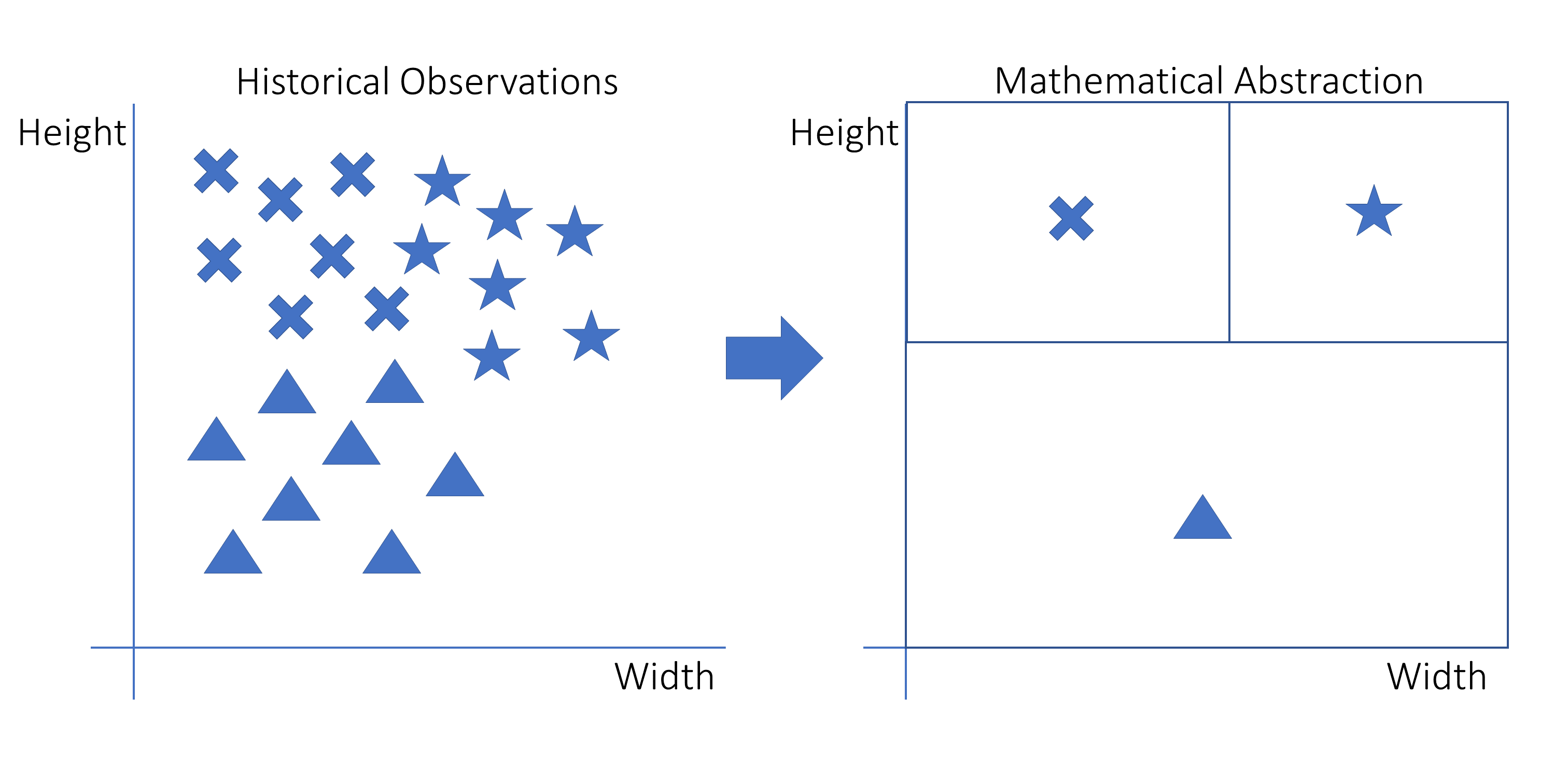
This graph is a visual representation of a machine learning model that is fitted onto historical data. On the left are the original observations with three variables: height, width, and shape. The shapes are stars, crosses, and triangles.
The shapes are located in different areas of the graph. On the right, you see how those original observations have been translated to a decision rule. For a new observation, you need to know the width and the height to determine in which square it falls. The square in which it falls, in turn, defines which shape it is most likely to have.
Many different models could be used for this task. A model is a mathematical formula that can be used to describe data points. One example is the linear model, which uses a linear function defined by the formula y = ax + b.
If you estimate, or fit, a model, you find the optimal values for the fixed parameters using some algorithm. In the linear model, the parameters are a and b. Luckily, you won’t have to invent such estimation algorithms to get started. They’ve already been discovered by great mathematicians.
Once the model is estimated, it becomes a mathematical formula in which you can fill in values for your independent variables to make predictions for your target variable. From a high-level perspective, that’s all that happens!
Distinguishing Features of kNN
Now that you understand the basic idea behind machine learning, the next step is understanding why there are so many models available. The linear model that you just saw is called linear regression.
Linear regression works in some cases but doesn’t always make very precise predictions. That’s why mathematicians have come up with many alternative machine learning models that you can use. The k-Nearest Neighbors algorithm is one of them.
All these models have their peculiarities. If you work on machine learning, you should have a deep understanding of all of them so that you can use the right model in the right situation. To understand why and when to use kNN, you’ll next look at how kNN compares to other machine learning models.
kNN Is a Supervised Machine Learning Algorithm
The first determining property of machine learning algorithms is the split between supervised and unsupervised models. The difference between supervised and unsupervised models is the problem statement.
In supervised models, you have two types of variables at the same time:
- A target variable, which is also called the dependent variable or the
yvariable. - Independent variables, which are also known as
xvariables or explanatory variables.
The target variable is the variable that you want to predict. It depends on the independent variables and it isn’t something that you know ahead of time. The independent variables are variables that you do know ahead of time. You can plug them into an equation to predict the target variable. In this way, it’s relatively similar to the y = ax + b case.
In the graph that you’ve seen before and the following graphs in this section, the target variable is the shape of the data point, and the independent variables are height and width. You can see the idea behind supervised learning in the following graph:
Read the full article at https://realpython.com/knn-python/ »
[ Improve Your Python With 🐍 Python Tricks 💌 – Get a short & sweet Python Trick delivered to your inbox every couple of days. >> Click here to learn more and see examples ]
from Real Python
read more


No comments:
Post a Comment