Stochastic Gradient Descent Algorithm With Python and NumPy

Stochastic gradient descent is an optimization algorithm often used in machine learning applications to find the model parameters that correspond to the best fit between predicted and actual outputs. It’s an inexact but powerful technique.

Stochastic gradient descent is widely used in machine learning applications. Combined with backpropagation, it’s dominant in neural network training applications.

In this tutorial, you’ll learn:

• How gradient descent and stochastic gradient descent algorithms work
• How to apply gradient descent and stochastic gradient descent to minimize the loss function in machine learning
• What the learning rate is, why it’s important, and how it impacts results
• How to write your own function for stochastic gradient descent

Free Bonus: 5 Thoughts On Python Mastery, a free course for Python developers that shows you the roadmap and the mindset you’ll need to take your Python skills to the next level.

Basic Gradient Descent Algorithm

The gradient descent algorithm is an approximate and iterative method for mathematical optimization. You can use it to approach the minimum of any differentiable function.

Note: There are many optimization methods and subfields of mathematical programming. If you want to learn how to use some of them with Python, then check out Scientific Python: Using SciPy for Optimization and Hands-On Linear Programming: Optimization With Python.

Although gradient descent sometimes gets stuck in a local minimum or a saddle point instead of finding the global minimum, it’s widely used in practice. Data science and machine learning methods often apply it internally to optimize model parameters. For example, neural networks find weights and biases with gradient descent.

Cost Function: The Goal of Optimization

The cost function, or loss function, is the function to be minimized (or maximized) by varying the decision variables. Many machine learning methods solve optimization problems under the surface. They tend to minimize the difference between actual and predicted outputs by adjusting the model parameters (like weights and biases for neural networks, decision rules for random forest or gradient boosting, and so on).

In a regression problem, you typically have the vectors of input variables 𝐱 = (𝑥₁, …, 𝑥ᵣ) and the actual outputs 𝑦. You want to find a model that maps 𝐱 to a predicted response 𝑓(𝐱) so that 𝑓(𝐱) is as close as possible to 𝑦. For example, you might want to predict an output such as a person’s salary given inputs like the person’s number of years at the company or level of education.

Your goal is to minimize the difference between the prediction 𝑓(𝐱) and the actual data 𝑦. This difference is called the residual.

In this type of problem, you want to minimize the sum of squared residuals (SSR), where SSR = Σᵢ(𝑦ᵢ − 𝑓(𝐱ᵢ))² for all observations 𝑖 = 1, …, 𝑛, where 𝑛 is the total number of observations. Alternatively, you could use the mean squared error (MSE = SSR / 𝑛) instead of SSR.

Both SSR and MSE use the square of the difference between the actual and predicted outputs. The lower the difference, the more accurate the prediction. A difference of zero indicates that the prediction is equal to the actual data.

SSR or MSE is minimized by adjusting the model parameters. For example, in linear regression, you want to find the function 𝑓(𝐱) = 𝑏₀ + 𝑏₁𝑥₁ + ⋯ + 𝑏ᵣ𝑥ᵣ, so you need to determine the weights 𝑏₀, 𝑏₁, …, 𝑏ᵣ that minimize SSR or MSE.

In a classification problem, the outputs 𝑦 are categorical, often either 0 or 1. For example, you might try to predict whether an email is spam or not. In the case of binary outputs, it’s convenient to minimize the cross-entropy function that also depends on the actual outputs 𝑦ᵢ and the corresponding predictions 𝑝(𝐱ᵢ):

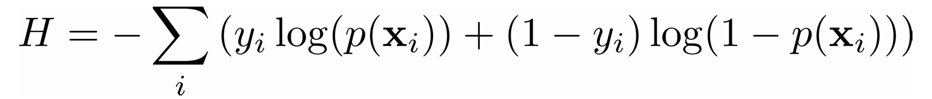
In logistic regression, which is often used to solve classification problems, the functions 𝑝(𝐱) and 𝑓(𝐱) are defined as the following:

Again, you need to find the weights 𝑏₀, 𝑏₁, …, 𝑏ᵣ, but this time they should minimize the cross-entropy function.

Gradient of a Function: Calculus Refresher

In calculus, the derivative of a function shows you how much a value changes when you modify its argument (or arguments). Derivatives are important for optimization because the zero derivatives might indicate a minimum, maximum, or saddle point.

The gradient of a function 𝐶 of several independent variables 𝑣₁, …, 𝑣ᵣ is denoted with ∇𝐶(𝑣₁, …, 𝑣ᵣ) and defined as the vector function of the partial derivatives of 𝐶 with respect to each independent variable: ∇𝐶 = (∂𝐶/∂𝑣₁, …, ∂𝐶/𝑣ᵣ). The symbol ∇ is called nabla.

The nonzero value of the gradient of a function 𝐶 at a given point defines the direction and rate of the fastest increase of 𝐶. When working with gradient descent, you’re interested in the direction of the fastest decrease in the cost function. This direction is determined by the negative gradient, −∇𝐶.

Read the full article at https://realpython.com/gradient-descent-algorithm-python/ »

---

[ Improve Your Python With 🐍 Python Tricks 💌 – Get a short & sweet Python Trick delivered to your inbox every couple of days. >> Click here to learn more and see examples ]

from Real Python
read more