Thursday, December 31, 2020

Israel Fruchter: Taking Github Actions for a walk in the park

Taking Github Actions for a walk in the park

Travis started to scare me a bit

People were talking about github actions for a while now, lot of hype around it. I myself was quite happy with the things I’ve managed to get done with Travis.

But then came in this announcement from travis: “The new pricing model for travis-ci.com”. I was reading via lot of the backlash in tweeter about it, and after carefully reading the announcement itself, I was starting to think that the work I did for scylla-driver was counting on Travis too much.

Recently I’ve start seeing long queues for job triggers in travis, and I was starting to have second thoughts about picking travis. (not so long ago, less than a year ago)

The sweet setup I had in Travis

As a recap for scylla-driver, since it’s a c based package, heavily using cython. We are building python wheels for windows, mac, linux, ranging from python2.7 to python3.9, and pypy. (also using the Travis experimental aarch64 and ppc64le support)

For building the wheels we are using cibuildwheel, which is a nifty tool that magically keep all know how, on how building wheels correctly on multiple platforms. In linux, it’s using the official docker images provided by the [Python Packaging Authority ] for manylinux2014. And on windows and mac equivalents with the correct set to needed tool to get you wheel happily containing all the need dynamic libraries it depended on

cibuildwheel also comes with readily available examples for all the major CI system out there

cibuildwheel is also helping you in running unittest ontop of each built wheel (since in my case the setup is a bit complex, getting it installed and compile across the board was hard, we we’re skipping some unittest on some platforms)

Travis was also running our integration test suite, and running it on our PRs, and automatically uploading all the wheels and source distribution to Pypi.

I was working on this setup for long week, with a tight deadline for it to be ready for europython2020, thanks to @ultrabug

Github actions

For a while I was a bit unsure if it would be a match to what I had in travis. But one day our own Jenkins server was down for maintenance, and a big portion of my day was clear case of that.

I’ve started with copy-pasting cibuildwheel github actions example, and worked my way from there.

When I’ve started adding all the different unittest and platforms, I was struggling a bit with how the matrix is working, and how conditional steps works.

It ended up something like this, almost identical to what I had in travis:

name: Build and upload to PyPi

on: [push, pull_request]

env:
  ...

jobs:
  build_wheels:
    name: Build wheels $ ($)
    if: contains(github.event.pull_request.labels.*.name, 'test-build') || github.event_name == 'push' && endsWith(github.event.ref, 'scylla')
    runs-on: $
    strategy:
      fail-fast: false
      matrix:
        include:
          - os: ubuntu-18.04
            platform: x86_64

          - os: ubuntu-18.04
            platform: i686

          - os: ubuntu-18.04
            platform: PyPy

          - os: windows-latest
            platform: win32

          - os: windows-latest
            platform: win64

          - os: windows-latest
            platform: PyPy

          - os: macos-latest
            platform: all

          - os: macos-latest
            platform: PyPy

We had a nice twist that we didn’t have before, but now we can control from github PR which part of my pipeline would run using label, since github actions is so tightly integrated you can lookup almost anything related to the PR.

Github Actions - UI

This is how the final thing looks like:

logging is a bit weird to watch while it’s running, but after the fact the log are very tidy to look at

Late surprise - cross compile using qemu

With almost perfect timing I’ve run into this https://ift.tt/380SGhY by Pavel Savchenko

I was trying all kind of things to get aarch64 support, but this PR figure it out quite nicely, with one magic step:

- name: Set up QEMU
id: qemu
uses: docker/setup-qemu-action@v1
with:
    platforms: all

For reference the full workflow

Now we can have docker using qemu to run docker instances based on different cpu architecture, it’s horribly slow but it’s working.

And nice side effect I’ve learned how to run it locally, so I can debug those things. Something I haven’t figured when running with Travis, apparently travis was using the same trick on their experimental support for those architectures.

Summary

Github actions works out of the box, with almost zero fraction, almost anything I could think about I’ve found a readily available step I can pickup, very impressing.

One thing I haven’t yet tried out, is using self hosted runner, hopefully I won’t need it. Cause who want to babysit anther server on his own, or worse, a bunch of them.


from Planet Python
via read more

Sumana Harihareswara - Cogito, Ergo Sumana: MOSS Video, BSSw Honorable Mention, and The Maintainership Book I Am Writing

Video

Mozilla interviewed me about the Python Package Index (PyPI), a USD$170,000 Mozilla Open Source Support award I helped the Python Software Foundation get in 2017, and how we used that money to revamp PyPI and drive it forward in 2017 and 2018.

From that interview, they condensed a video (2 minutes, 14 seconds) featuring, for instance, slo-mo footage of me making air quotes. Their tweet calls me "a driving force behind" PyPI, and given how many people were working on it way before I was, that's quite a compliment!

I will put a transcript in the comments of this blog post.

(Please note that they massively condensed this video from 30+ minutes of interview. In the video, I say, "the site got popular before the code got good". In the interview, I did not just say that without acknowledging the tremendous effort of past volunteers who worked on the previous iteration of PyPI and kept the site going through massive infrastructure challenges, but that's been edited (for brevity, I assume).)

This video is the first in a series meant to encourage people to apply for MOSS funding. I mentioned MOSS in my grants roundup last month. If you want to figure out whether to apply for MOSS funding for your open source software project, and you need help, ping me for a free 20-minute chat or phone call and I can give you some quick advice. (Offer limited in case literally a hundred people contact me, which is unlikely.)

BSSw

The Better Scientific Software (BSSw) Fellowship Program "gives recognition and funding to leaders and advocates of high-quality scientific software." I'm one of three Honorable Mentions for 2020.

The main goal of the BSSw Fellowship program is to foster and promote practices, processes, and tools to improve developer productivity and software sustainability of scientific code. We also anticipate accumulating a growing community of BSSw Fellowship alums who can serve as leaders, mentors, and consultants to increase the visibility of those involved in scientific software production and sustainability in the pursuit of scientific discovery.

Exascale Computing Project logoThat's why I'll be at the Exascale Computing Project Annual Meeting next week in Houston, so if you're there, I hope to meet you. In particular I'd like to meet the leaders of open source projects who want help streamlining contribution processes, growing more maintainers, managing communications with stakeholders, participating in internship projects like Google Summer of Code and Outreachy, expediting releases, and getting more out of hackathons. My consulting firm provides these services, and at ECPAM I can give you some free advice.

Book

And here's the project I'm working on -- why I received this honor.

In 2020, I am writing the first draft of a book teaching the skills open source software maintainers need, aimed at those working scientists and other contributors who have never managed public-facing projects before.

More than developer time, maintainership -- coordination, leadership, and management -- is a bottleneck in software sustainability. The lack of skilled managers is a huge blocker to the sustainability of Free/Libre Open Source Software (FLOSS) infrastructure.

Many FLOSS project maintainers lack management experience and skill. This textbook/self-help guide for new and current maintainers of existing projects ("brownfield projects") will focus on teaching specific project management skills in the context of FLOSS. This will provide scalable guidance, enabling existing FLOSS contributors to become more effective maintainers.

Existing "how to run a FLOSS project" documentation (such as Karl Fogel's Producing Open Source Software) addresses fresh-start "greenfield" projects rather than more common "brownfield", and doesn't teach specific project management skills (e.g., getting to know a team, creating roadmaps, running asynchronous meetings, managing budgets, and writing email memos). Existing educational pathways for scientists and developers (The Carpentries, internships and code schools) don't cover FLOSS-specific management skills.

So I'm writing a sequel to Karl's book -- with his blessing -- and I'm excited to see how I can more scalably share the lessons I've learned in more than a decade of leading open source projects.

I don't yet have a full outline, a publisher, or a length in mind. I'll be posting more here as I grow my plans. Thanks to BSSw and all my colleagues and friends who have encouraged me.


from Planet Python
via read more

The Best Posts in 2020 – Neptune’s Blog Summary

It’s the last day of the year, so we decided to go with the end-of-the-year flow and create our own blog summary!...

The post The Best Posts in 2020 – Neptune’s Blog Summary appeared first on neptune.ai.


from Planet SciPy
read more

Matt Layman: Customer Docs - Building SaaS #85

In this episode, I integrated customer documentation into the app. I showed how to build Sphinx documentation into a Django project, then created a help view to link to the docs. Finally, I added documentation building to the deployment process. I previously created a Sphinx documentation project to hold docs for my app, but I had not hooked the docs into my project yet. Before hooking it in, I explained how Sphinx works and how I customized the documentation to fit with my project.

from Planet Python
via read more

PyPy Development: Mac meets Arm64

Looking for sponsorship

Apple now ships Macs which are running on an arm64 variant machine with the latest version of MacOS, Big Sur M1. We are getting requests for PyPy to support this new architecture. Here is our position on this topic (or at least mine, Armin Rigo's), and how you can help.

Porting PyPy is harder than just re-running the compiler, because PyPy contains a few big architecture-dependent "details", like the JIT compiler and the foreign function interfaces (CFFI and ctypes).

Fixing the JIT compiler should not be too much work: we already support arm64, just the Linux one. But Apple made various details different (like the calling conventions). A few other parts need to be fixed too, notably CFFI and ctypes, again because of the calling conventions.

Fixing that would be a reasonable amount of work. I would do it myself for a small amount of money. However, the story doesn't finish here. Obviously, the start of the story would be to get ssh access to a Big Sur M1 machine. (If at this point you're thinking "sure, I can give you ssh access for three months", then please read on.) The next part of the story is that we need a machine available long term. It can be either a machine provided and maintained by a third party, or alternatively a pot of money big enough to support the acquision of a machine and ongoing work of one of us.

If we go with the provided-machine solution: What we need isn't a lot of resources. Our CI requires maybe 10 GB of disk space, and a few hours of CPU per run. It should fit into 8 GB of RAM. We normally do a run every night but we can certainly lower the frequency a bit if that would help. However, we'd ideally like some kind of assurance that you are invested into maintaining the machine for the next 3-5 years (I guess, see below). We had far too many machines that disappeared after a few months.

If we go with the money-supported solution: it's likely that after 3-5 years the whole Mac base will have switched to arm64, we'll drop x86-64 support for Mac, and we'll be back to the situation of the past where there was only one kind of Mac machine to care about. In the meantime, we are looking at 3-5 years of lightweight extra maintenance. We have someone that has said he would do it, but not for free.

If either of these two solutions occurs, we'll still have, I quote, "probably some changes in distutils-type stuff to make python happy", and then some packaging/deployment changes to support the "universal2" architecture, i.e. including both versions inside a single executable (which will not be just an extra switch to clang, because the two versions need a different JIT backend and so must be translated separately).

So, now all the factors are on the table. We won't do the minimal "just the JIT compiler fixes" if we don't have a plan that goes farther. Either we get sufficient money, and maybe support, and then we can do it quickly; or PyPy will just remain not natively available on M1 hardware for the next 3-5 years. We are looking forward to supporting M1, and view resources contributed by the community as a vote of confidence in assuring the future of PyPy on this hardware. Contact us: pypy-dev@python.org, or our private mailing list pypy-z@python.org.

Thanks for reading!

Armin Rigo


from Planet Python
via read more

PyCharm: PyCharm 2020.3.2 Supports Apple Silicon

We have special news for those of you using Mac with an M1 chip: PyCharm 2020.3.2 is out and brings support for Apple Silicon!

To start working, download the separate installer for PyCharm for Apple Silicon from our website or via the Toolbox App (under the Available for Apple M1 section). Please note that a previously installed PyCharm version running via Rosetta2 will not update to run natively.

Update now and share your feedback with us!

Other significant fixes in 2020.3.2 include:

  • PyCharm supports debugging for Jupyter notebooks. Using Alt + Shift + Enter (or Option + Shift + Enter for Mac), you can do cell-by-cell debugging. We fixed the issue with freezes after resuming the debugging process, so it now works smoothly.
  • An issue that was breaking the helpers path and preventing WSL debugger from working is now fixed.
  • Unused variables sometimes arise in complex assignments. The “Unused local” code inspection identifies such cases and suggests a quick-fix: Remove unused variable. Press Alt + Enter (or Option + Enter for Mac) to see the suggestion and accept it. The quick-fix now removes only the unused variable, not the entire statement.
  • PyCharm detects when you are trying to import a non-existing name in CapitalizedWords style. Now PyCharm defines such an identifier as a class and suggests an appropriate quick-fix: “Create class … in module …”. To use the quick-fix, click the lightbulb or press Alt + Enter (or Option + Enter for Mac).

For other resolved issues, refer to the release notes. Please comment on this post or report your suggestions to our issue tracker.


from Planet Python
via read more

Wednesday, December 30, 2020

Python Morsels: Python's Two Different String Representations

Transcript:

Let's talk about the two different string representations that all Python objects have.

String Representation of an Object

We have a datetime.date object here that represents the Python 2 end of life date:

>>> from datetime import date
>>> eol = date(2020, 1, 1)

If we type eol from a Python shell, we're gonna see something that looks kind of like the code that I originally typed in to get that object:

>>> eol
datetime.date(2020, 1, 1)

If we print out this datetime.date object, we instead see something that looks more like a human-readable date:

>>> print(eol)
2020-01-01

When we called print, it actually called the built-in str function to get this string representation:

>>> str(eol)
'2020-01-01'

This is the human-readable string representation for this object.

Likewise, typing just eol at the Python REPL also resulted in a built-in function being called, the repr function:

>>> repr(eol)
'datetime.date(2020, 1, 1)'

This is the programmer-readable string representation for this object.

The human-readable string representation is the thing that an end-user of our program might want to see, which is the reason that it's what we get when we print something out.

The programmer-readable string representation is what another Python programmer might want to see, which is the reason that we see it when we're playing around with objects at the Python REPL.

More on the Programmer Readable Representation

If we look at help on the built-in repr function, we will see that many objects, including most of the built-ins, use a particular convention for the programmer-readable string representation:

>>> help(repr)
Help on built-in function repr in module builtins:

repr(obj, /)
    Return the canonical string representation of the object.

    For many object types, including most builtins, eval(repr(obj)) == obj.

>>>

This convention says that the string that you get back, should actually be the Python code which if you were to execute it, would give you an object that would be equivalent to the object you started with.

So what that really means is, the result of typing just eol at the REPL should represent something that if we would execute that code, it would give us back basically the same date object:

>>> eol
datetime.date(2020, 1, 1)

Most Objects Only Have a Programmer-Readable String Representation

Now, we should note that most Python objects actually only have one string representation.

The one-string representation they have is the programmer-readable one.

So if we take a list, a dictionary, an integer, a floating-point number, or most objects in Python, and we convert them to a string, we see something that looks like Python code:

>>> numbers = [2, 1, 3, 4, 7]
>>> str(numbers)
'[2, 1, 3, 4, 7]'

If we call the built-in repr function on them, we'll see the same thing:

>>> repr(numbers)
'[2, 1, 3, 4, 7]'
>>> print(numbers)
[2, 1, 3, 4, 7]
>>> numbers
[2, 1, 3, 4, 7]

Most objects in Python do not have a human-readable string representation. They're meant to be used by other Python programmers, they're not necessarily meant to be printed out.

Summary

So in Python, we have two different string representations. str is the human-readable string representation, if that exists.

If it doesn't exist, the built-in str function, will call the built-in repr function, which gives you the programmer-readable string representation, which is meant for other Python programmers.

If you're converting something to a string, the str function is a pretty great way to do it. But if you specifically want a string representation of an object that's meant for another Python programmer, you might want to use the built-in repr function.


from Planet Python
via read more

Test and Code: 141: Visual Testing - Angie Jones

Visual Testing has come a long way from the early days of x,y mouse clicks and pixel comparisons. Angie Jones joins the show to discuss how modern visual testing tools work and how to incorporate visual testing into a complete testing strategy.

Some of the discussion:

  • Classes of visual testing:
    • problems with pixel to pixel testing
    • DOM comparisons, css, html, etc.
    • AI driven picture level testing, where failures look into the DOM to help describe the problem.
  • Where visual testing fits into a test strategy.
  • Combining "does this look right" visual testing with other test workflows.
  • "A picture is worth a thousand assertions" - functional assertions built into visual testing.
  • Baselining pictures in the test workflow.

Also discussed:

  • automation engineer
  • Test Automation University

Special Guest: Angie Jones.

Sponsored By:

Support Test & Code : Python Testing for Software Engineering

Links:

<p>Visual Testing has come a long way from the early days of x,y mouse clicks and pixel comparisons. Angie Jones joins the show to discuss how modern visual testing tools work and how to incorporate visual testing into a complete testing strategy. </p> <p>Some of the discussion:</p> <ul> <li>Classes of visual testing: <ul> <li>problems with pixel to pixel testing</li> <li>DOM comparisons, css, html, etc.</li> <li>AI driven picture level testing, where failures look into the DOM to help describe the problem. </li> </ul></li> <li>Where visual testing fits into a test strategy.</li> <li>Combining &quot;does this look right&quot; visual testing with other test workflows.</li> <li>&quot;A picture is worth a thousand assertions&quot; - functional assertions built into visual testing.</li> <li>Baselining pictures in the test workflow.</li> </ul> <p>Also discussed:</p> <ul> <li>automation engineer</li> <li>Test Automation University</li> </ul><p>Special Guest: Angie Jones.</p><p>Sponsored By:</p><ul><li><a href="https://ift.tt/2JDHRTz" rel="nofollow">PyCharm Professional</a>: <a href="https://ift.tt/2JDHRTz" rel="nofollow">Try PyCharm Pro for 4 months and learn how PyCharm will save you time.</a> Promo Code: TESTANDCODE20</li></ul><p><a href="https://ift.tt/2tzXV5e" rel="payment">Support Test & Code : Python Testing for Software Engineering</a></p><p>Links:</p><ul><li><a href="https://ift.tt/2zGdHN4" title="Test Automation University" rel="nofollow">Test Automation University</a></li></ul>

from Planet Python
via read more

Disnatia X/Potências de X

Nenhuma equipe de heróis me é tão querida quanto X-Men. Lá pelo final dos anos 90 comecei a colecionar por alguns anos, mas em seguida veio o fatídico aumento de preço com as Super-Heróis Premium, o que me acabou desmotivando a comprar. De lá para cá, acompanho esporadicamente, lendo notícias sobre, comprando uma ou outra… Continue a ler »Disnatia X/Potências de X

from Planet SciPy
read more

The Open Sourcerer: Blogging about Python desktop apps improvements on Planet Python

Hi, fellow pythonistas! Before I start publishing future Python-related posts to this aggregator, I would like to shortly introduce myself and the reason for this blog’s presence on the planet.


I am a business management consultant, but I am also, in my spare time, an independent free & open-source software developer, designer and maintainer who happens to use Python as his sole programming language. I created Specto (all Python) many years ago, I co-maintained the Pitivi video editor (also written in Python) for many years, and nowadays I co-maintain GTG which is, you guessed it, another “pure Python” free & open-source desktop application. It looks like this:

Here I blog mainly about new releases and improvements in my Python software apps (which means GTG lately, but I also have a couple of pythonic utility apps I’ve been meaning to publish sometime soon), and sometimes write about performance optimization in software applications in general, or how a particular bug was solved. As such, my blog posts tend to be “applied Python” type of content rather than theoretical tutorial-style blog posts.

I believe that successful Python application improvements & releases serve as tangible proof of Python’s power as a desktop GUI application development technology that can attract healthy contributor communities. It is not every day you see a project come back to life like what we did with GTG, and I hope this well-designed, practical, cornerstone desktop application can serve as a success story for Python on the desktop.

In recent days, I have also started working for the Montréal Polytechnique university’s neuroimaging laboratory/research group, where I help them structure their documentation and scientific communication efforts to the public. Their neuroimaging software projects are typically written in Python, so if there is some interest in that (?), and should I find topics that seem relevant to talk about on my blog, I may write about that too (but I’m no neuroscientist!)


I look forward to contributing to Planet Python, and if you’re curious about the broader topics I blog about, I also have a posts notification mailing list, and on Twitter you can also find me, GTG, Pitivi, the PolyMTL Neuro lab account, and the accounts of the lab’s biggest pythonic apps as well.


from Planet Python
via read more

Applications of AI in Drone Technology: Building Machine Learning Models That Work on Drones (With Tensorflow/Keras)

Welcome back to the second part of Building a Facemask Surveillance System with Drone Technology and Deep Learning. In the first part,...

The post Applications of AI in Drone Technology: Building Machine Learning Models That Work on Drones (With Tensorflow/Keras) appeared first on neptune.ai.


from Planet SciPy
read more

Tuesday, December 29, 2020

Matthew Wright: Indexing and Selecting in pandas – slicing

Slicing data in pandas This is second in the series on indexing and selecting data in pandas. If you haven't read it yet, see the first post that covers the basics of selecting based on index or relative numerical indexing. In this post, I'm going to review slicing, which is a core Python topic, but has … Continue reading Indexing and Selecting in pandas – slicing


from Planet Python
via read more

Mike Driscoll: Python Image Processing Kickstarter Coming Next Week!

I will be launching a new Kickstarter on Monday, January 4th to help launch my 9th book, Pillow: Image Processing with Python.

In this book, you will learn how to edit photos with Python. You will discover how to extract metadata, crop, apply filters, resize and so much more!

Pillow: Image Processing with Python Kickstarter
Here is the high-level table of contents:

  • Chapter 1 – Pillow Basics
  • Chapter 2 – Colors
  • Chapter 3 – Getting Image Metadata (ExifTags / TiffTags)
  • Chapter 4 – Image Filters
  • Chapter 5 – Cropping, Rotating & Resizing Images
  • Chapter 6 – Enhancing Images (ImageEnhance)
  • Chapter 7 – Combining Images
  • Chapter 8 – Drawing with Pillow (ImageDraw)
  • Chapter 9 – ImageChops
  • Chapter 10 – Pillow Integration with GUIs
Note: This table of contents is subject to change. Chapters may be re-ordered, renamed, added, or deleted as the author sees fit.

You can preview and follow the Kickstarter now!

The post Python Image Processing Kickstarter Coming Next Week! appeared first on Mouse Vs Python.


from Planet Python
via read more

Python Anywhere: Brexit update

PythonAnywhere is a UK-based company, and the transition period for the UK’s exit from the European Union on will end on 31 December 2020. This will not have any visible effect for people who use our free service. For our paying customers outside the EU, including in the UK, there will also be no changes.

For paying customers inside the EU, the only effect should be that you’ll receive two billing reminders for January, a “pro-forma” one that will come at the usual time, just before your monthly payment is made, and another one later on in the month, which will be the formal “VAT invoice” required by EU tax law.

You will, of course, only be charged once; the second billing reminder will just provide some extra tax information. The remainder of this post is the details of why those two billing reminders will be sent, and we’re posting it here for those who like reading about tax laws…


from Planet Python
via read more

Zero to Mastery: Python Monthly 💻🐍 December 2020

13th issue of Python Monthly! Read by 20,000+ Python developers every month. This monthly newsletter is focused on keeping you up to date with the industry, keeping your skills sharp, without wasting your valuable time.

from Planet Python
via read more

PyCoder’s Weekly: Issue #453 (Dec. 29, 2020)

#453 – DECEMBER 29, 2020
View in Browser »

The PyCoder’s Weekly Logo


Accelerating Python on GPUs With nvc++ and Cython

Python on GPUs has become a big topic for processing big data and scientific computing. In this article from the NVIDIA Developer Blog, you’ll learn how to leverage C++ in Python using Cython and the nvc++ library. There’s even a real-world example that illustrates the Jacobi method to solve a heat equation.
ASHWIN SRINATH

Create Codeless Automation, Get Python Script!

alt

From now on, any test created using TestProject’s automation platform can be generated into Python code, fully compatible with Appium & Selenium. Simply record your test, export to Python & continue from there! No complicated setups - one executable does all the heavy lifting for you. Try it today →
TESTPROJECT sponsor

We Downloaded 10,000,000 Jupyter Notebooks From Github: This Is What We Learned

The JetBrains Datalore team downloaded ten million Jupyter Notebooks and analyzed them to determine things like which languages were the most popular, what kinds of content are in notebook cells, and how consistently notebooks can be reproduced. It’s a fascinating look into trends in data science technology!
ALENA GUZHARINA

Django Admin Customization

Learn how to customize Django’s admin with Python. You’ll use AdminModel objects to add display columns, calculate values, link to referring objects, and search and filter results. You’ll also use template overriding to gain full control over the admin’s HTML.
REAL PYTHON course

Unravelling Boolean Operations

In the latest entry to his series on syntactic sugar, Brett Cannon explores boolean expressions. You’ll learn how boolean expressions “short circuit” and, as an unexpected bonus, a peek into how CPython “cheats” at variables.
BRETT CANNON

Top 10 Python Libraries of 2020 You Should Know About

This listicle is full of Python projects that you really should know about! Each library on the lists was launched or popularized in 2020 and has seen steady maintenance since its launch. Lots of great projects here!
ALAN DESCOINS

2020 Real Python Articles in Review

It’s been quite the year! The Real Python team has written, edited, curated, illustrated, and produced a mountain of Python articles this year. This year-end wrap-up shares a collection of articles that showcase a diversity of Python topics.
REAL PYTHON

Discussions

How Do You Pronounce “Char”?

Charcoal? Chair? Car? Tupple? Two Pull? Sequel? Squeal? Why not end the year with a hearty discussion about pronunciation? (By the way… it’s “care.”)
REDDIT

Python Jobs

Entry-Level Engineering Programme (London, UK)

Tessian

Senior Backend Engineer (London, UK)

Tessian

Backend Engineer (London, UK)

Tessian

Advanced Python Engineer (Newport Beach, CA, USA)

Research Affiliates

More Python Jobs >>>

Articles & Tutorials

NumPy Illustrated: The Visual Guide to NumPy

This illustrated guide to NumPy is a great way to learn NumPy or brush up on the package. Full of great visual aides, this tutorial covers all the basics and more!
LEV MAXIMOV

Isolate Python Subinterpreters

In this post, Victor Stinner takes a look back at the progress made on isolating Python subinterpreters in 2019 and 2020. You’ll learn about the technical challenges that have been solved, the current status of the project, and what the future holds.
VICTOR STINNER

Level Up Your Python Skills: PSF Charity Sale (Ends Jan 1)

alt

Support the Python Software Foundation and level up your Python skills with books, courses, and more. You’ll get a discount on Python training products, and the money raised in this fundraiser will help the PSF fund the tools and initiatives that Pythonistas use everyday.
REAL PYTHON sponsor

The Zen of Python: A Most in Depth Article

Claiming to be “the most in-depth article about the Zen of Python,” this post covers the history of the Zen as told through comments from Guido van Rossum, Tim Peters, Barry Warsaw, and other Python heavyweights.
ABDUR-RAHMAAN JANHANGEER

Python and MySQL Database: A Practical Introduction

Learn how to connect your Python application with a MySQL database. You’ll design a movie rating system and perform some common queries on it. You’ll also see best practices and tips to prevent SQL injection attacks.
REAL PYTHON

Indexing and Selecting in Pandas

Selecting and indexing items from pandas Series and DataFrame objects can be confusing. This article gives you a lucid breakdown of three ways to select elements from pandas objects and explains the differences between each one.
MATT WRIGHT

Web Authentication Methods Compared

Take a look at commonly used methods for handling web authentication for Python web development including the pros and cons of each method. You’ll see how to apply different methods to the Flask, Django, and FastAPI frameworks.
AMAL SHAJI • Shared by Amal Shaji

Validating Data in Python With Cerberus

Thanks to an Advent of Code challenge, author Hector Castro was exposed to the Cerberus Python package for data validation. Get a quick introduction to Cerberus and see Hector’s solution to an Advent of Code challenge in this quick-yet-informative read.
HECTOR CASTRO

The Joy of Typed Python

The mypy project brings static type checking to Python. This opinion piece explores the good and the bad of typed Python from the perspective of someone who wouldn’t grab Python for their day-to-day coding.
BALAJEE RAMACHANDRAN opinion

Projects & Code

Events

Python Pizza New Year’s Party

December 31 to January 1, 2021
PYTHON.PIZZA

BelPy

January 30 – 31, 2021
BELPY.IN

PyCascades 2021 (Virtual)

February 19 – 21, 2021
PYCASCADES.COM

PyCon 2021 (Virtual)

May 12 – 18, 2021
PYCON.ORG


Happy Pythoning!
This was PyCoder’s Weekly Issue #453.
View in Browser »

alt

[ Subscribe to 🐍 PyCoder’s Weekly 💌 – Get the best Python news, articles, and tutorials delivered to your inbox once a week >> Click here to learn more ]


from Planet Python
via read more

Adversarial Attacks on Neural Networks: Exploring the Fast Gradient Sign Method

Since their invention, neural networks have always been the crème de la crème of machine learning algorithms. They have driven most of...

The post Adversarial Attacks on Neural Networks: Exploring the Fast Gradient Sign Method appeared first on neptune.ai.


from Planet SciPy
read more

Real Python: Django Admin Customization

The Django framework comes with a powerful administrative tool called admin. You can use it out of the box to quickly add, delete, or edit any database model from a web interface. But with a little extra code, you can customize the Django admin to take your admin capabilities to the next level.

In this course, you’ll learn how to:

  • Add attribute columns in the model object list
  • Link between model objects
  • Add filters to the model object list
  • Make model object lists searchable
  • Modify the object edit forms
  • Override Django admin templates

[ Improve Your Python With 🐍 Python Tricks 💌 – Get a short & sweet Python Trick delivered to your inbox every couple of days. >> Click here to learn more and see examples ]


from Planet Python
via read more

Django Admin Customization

The Django framework comes with a powerful administrative tool called admin. You can use it out of the box to quickly add, delete, or edit any database model from a web interface. But with a little extra code, you can customize the Django admin to take your admin capabilities to the next level.

In this course, you’ll learn how to:

  • Add attribute columns in the model object list
  • Link between model objects
  • Add filters to the model object list
  • Make model object lists searchable
  • Modify the object edit forms
  • Override Django admin templates

[ Improve Your Python With 🐍 Python Tricks 💌 – Get a short & sweet Python Trick delivered to your inbox every couple of days. >> Click here to learn more and see examples ]


from Real Python
read more

Stack Abuse: Ultimate Guide to Heatmaps in Seaborn with Python

Introduction

A heatmap is a data visualization technique that uses color to show how a value of interest changes depending on the values of two other variables.

For example, you could use a heatmap to understand how air pollution varies according to the time of day across a set of cities.

Another, perhaps more rare case of using heatmaps is to observe human behavior - you can create visualizations of how people use social media, how their answers on surveys changed through time, etc. These techniques can be very powerful for examining patterns in behavior, especially for psychological institutions who commonly send self-assessment surveys to patients.

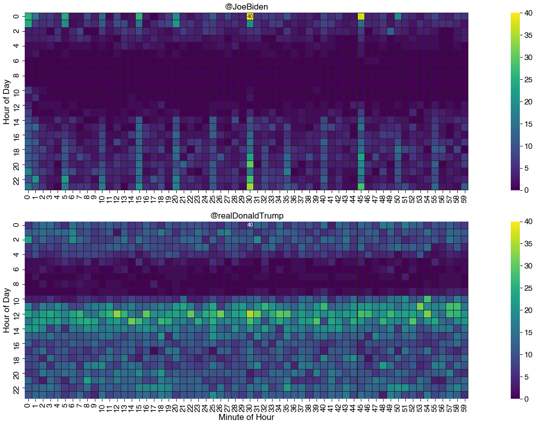
Here are two heatmaps that show the differences in how two users use Twitter:

heatmaps with seabornw

These charts contain all the main components of a heatmap. Fundamentally it is a grid of colored squares where each square, or bin, marks the intersection of the values of two variables which stretch along the horizontal and vertical axes.

In this example, these variables are:

  1. The hour of the day
  2. The minute of the hour

The squares are colored according to how many tweets fall into each hour/minute bin. To the side of the grid is a legend that shows us how the color relates to the count values. In this case, lighter (or warmer) colors mean more tweets and darker (or cooler) means fewer. Hence the name heatmap!

Heatmaps are most useful for identifying patterns in large amounts of data at a glance. For example, the darker, colder strip in the morning indicates that both candidates don't tweet much before noon. Also, the second user tweets much more frequently than the first user, with a sharper cut-off line at 10AM, whereas the first user doesn't have such a clear line. This can be attributed to personal scheduling during the day, where the second user typically finishes some assigned work by 10AM, followed by checking on social media and using it.

Heatmaps often make a good starting point for more sophisticated analysis. But it's also an eye-catching visualization technique, making it a useful tool for communication.

In this tutorial we will show you how to create a heatmap like the one above using the Seaborn library in Python.

Seaborn is a data visualization library built on top of Matplotlib. Together, they are the de-facto leaders when it comes to visualization libraries in Python.

Seaborn has a higher-level API than Matplotlib, allowing us to automate a lot of the customization and small tasks we'd typically have to include to make Matplotlib plots more suitable to the human eye. It also integrates closely to Pandas data structures, which makes it easier to pre-process and visualize data. It also has many built-in plots, with useful defaults and attractive styling.

In this guide, we'll cover three main sections:

  1. Data preparation
  2. Plotting a Heatmap
  3. Best Practices and Heatmap Customization

Let's get started!

Preparing a Dataset for Creating a Heatmap with Seaborn

Loading an Example Dataset with Pandas

Please note: This guide was written using Python 3.8, Seaborn 0.11.0, and Pandas 1.1.2.

For this guide, we will use a dataset that contains the timestamps of tweets posted by two of the 2020 U.S. presidential candidates at the time, Joe Biden and Donald Trump - between January 2017 and September 2020. A description of the dataset and how it was created can be found at here.

A fun exercise at home could be making your own dataset from your own, or friend's tweets and comparing your social media usage habits!

Our first task is to load that data and transform it into the form that Seaborn expects, and is easy for us to work with.

We will use the Pandas library for loading and manipulating data:

import pandas as pd

We can use the Pandas read_csv() function to load the tweet count dataset. You can either pass in the URL pointing to the dataset, or download it and reference the file manually:

data_url = "https://bit.ly/3cngqgL" # or "path/to/biden_trump_tweets.csv"
df = pd.read_csv(data_url, 
                 parse_dates=['date_utc'], 
                 dtype={'hour_utc':int,'minute_utc':int,'id':str}
                )

It's always worth using the head method to examine the first few rows of the DataFrame, to get familiar with its shape:

df.head()
id username date_utc hour_utc minute_utc retweets
0 815422340540547073 realDonaldTrump 2017-01-01 05:00:10+00:00 5 0 27134
1 815930688889352192 realDonaldTrump 2017-01-02 14:40:10+00:00 14 40 23930
2 815973752785793024 realDonaldTrump 2017-01-02 17:31:17+00:00 17 31 14119
3 815989154555297792 realDonaldTrump 2017-01-02 18:32:29+00:00 18 32 3193
4 815990335318982656 realDonaldTrump 2017-01-02 18:37:10+00:00 18 37 7337

Here, we've printed the first 5 elements in the DataFrame. We have the index of each row first, followed by the id of the tweet, the username of the user who tweeted that tweet, as well as time-related information such as the date_utc, hour_utc and minute_utc.

Finally, we've got the number of retweets at the end, which can be used to check for interesting relationship between the contents of the tweets and the "attention" it got.

Transforming the data into a wide-form DataFrame

It is common to find log data like this organized in a long (or tidy) form. This means there is a column for each variable, and each row of the data is a single observation (specific value) of those variables. Here, each tweet is each variable. Each row corresponds to one tweet and contains data about it.

But conceptually a heatmap requires that the data be organized in a short (or wide) form. And in fact the Seaborn library requires us to have the data in this form to produce heatmap visualizations like the ones we've seen before.

Wide-form data has the values of the independent variables as the row and column headings and the values of the dependent variable are contained in the cells.

This basically means we are using all the properties that we're not observing as categories. Keep in mind that some categories occur more than once. For example, in the original table, we have something like:

username hour_utc minute_utc
realDonaldTrump 12 4
realDonaldTrump 13 0
realDonaldTrump 12 4

Using the category principle, we can accumulate the occurrences of certain properties:

category occurrences
realDonaldTrump | 12 hours | 4 minutes 2
realDonaldTrump | 13 hours | 0 minutes 1

Which we can then finally transform into something more heatmap-friendly:

hours\minutes 0 1 2 3 4
12 0 0 0 0 2
13 1 0 0 0 0

Here, we've got hours as rows, as unique values, as well as minutes as columns. Each value in the cells is the number of tweet occurrences at that time. For example, here, we can see 2 tweets at 12:04 and one tweet at 13:01. With this approach, we've only got 24 rows (24 hours) and 60 columns. If you imagine this spread visually, it essentially is a heatmap, though, with numbers.

In our example I want to understand if there are any patterns to how the candidates tweet at different times of the day. One way to do this is to count the tweets created in each the hour of the day and each minute of an hour.

Technically, we've got 2880 categories. Each combination of the hour_utc, minute_utc and username is a separate category, and we count the number of tweet occurrences for each of them.

This aggregation is straight-forward using Pandas. The hour and the minute of creation are available in the columns hour_utc and minute_utc. We can use the Pandas groupby() function to collect together all the tweets for each combination of username, hour_utc, and minute_utc:

g = df.groupby(['hour_utc','minute_utc','username'])

This means that only rows that have the same value of hour_utc, minute_utc, username can be considered an occurrence of the same category.

Now we can count the number of tweets in each group by applying the nunique() function to count the number of unique ids. This method avoids double counting any duplicate tweets that might lurk in the data, if it's not cleaned properly beforehand:

tweet_cnt = g.id.nunique()

This gives us a Pandas Series with the counts we need to plot the heatmap:

tweet_cnt.head()
hour_utc  minute_utc  username       
0         0           JoeBiden           26
                      realDonaldTrump     6
          1           JoeBiden           16
                      realDonaldTrump    11
          2           JoeBiden            6
Name: id, dtype: int64

To transform this into the wide-form DataFrame needed by Seaborn we can use the Pandas pivot() function.

For this example, it will be easiest to take one user at a time and plot a heatmap for each of them separately. We can put this on a single figure or separate ones.

Use the Pandas loc[] accessor to select one users tweet counts and then apply the pivot() function. It uses unique values from the specified index/columns to form axes of the resulting DataFrame. We'll pivot the hours and minutes so that the resulting DataFrame has a wide-spread form:

jb_tweet_cnt = tweet_cnt.loc[:,:,'JoeBiden'].reset_index().pivot(index='hour_utc', columns='minute_utc', values='id')

Then take a peek at a section of the resulting DataFrame:

jb_tweet_cnt.iloc[:10,:9]
minute_utc 0 1 2 3 4 5 6 7 8
hour_utc
0 26.0 16.0 6.0 7.0 4.0 24.0 2.0 2.0 9.0
1 24.0 7.0 5.0 6.0 4.0 19.0 1.0 2.0 6.0
2 3.0 3.0 3.0 NaN 5.0 1.0 4.0 8.0 NaN
3 3.0 3.0 3.0 4.0 5.0 1.0 3.0 5.0 4.0
4 1.0 1.0 1.0 2.0 NaN NaN 1.0 1.0 1.0
5 1.0 2.0 NaN NaN NaN 1.0 NaN NaN NaN
6 NaN NaN NaN NaN NaN NaN NaN NaN NaN
10 7.0 2.0 1.0 NaN NaN NaN NaN NaN NaN
11 2.0 5.0 NaN NaN NaN NaN NaN NaN NaN
12 4.0 NaN 1.0 1.0 1.0 NaN 1.0 NaN NaN

Dealing with Missing Values

We can see above that our transformed data contains missing values. Wherever there were no tweets for a given minute/hour combination the pivot() function inserts a Not-a-Number (NaN) value into the DataFrame.

Furthermore pivot() does not create a row (or column) when there were no tweets at all for a particular hour (or minute).

See above where hours 7, 8 and 9 are missing.

This will be a common thing to happen when pre-processing data. Data might be missing, could be of odd types or entries (no validation), etc.

Seaborn can handle this missing data just fine, it'll just plot without them, skipping over hours 7, 8 and 9. However, our heatmaps will be more consistent and interpretable if we fill in the missing values. In this case we know that missing values are really a count of zero.

To fill in the NaNs that have already been inserted, use fillna() like so:

jb_tweet_cnt.fillna(0, inplace=True)

To insert missing rows - make sure all hour and minute combinations appear in the heatmap - we'll reindex() the DataFrame to insert the missing indices and their values:

# Ensure all hours in table
jb_tweet_cnt = jb_tweet_cnt.reindex(range(0,24), axis=0, fill_value=0)
# Ensure all minutes in table
jb_tweet_cnt = jb_tweet_cnt.reindex(range(0,60), axis=1, fill_value=0).astype(int) 

Great. Now we can complete our data preparation by repeating the same steps for the other candidates tweets:

dt_tweet_cnt = tweet_cnt.loc[:,:,'realDonaldTrump'].reset_index().pivot(index='hour_utc', columns='minute_utc', values='id')
dt_tweet_cnt.fillna(0, inplace=True)
dt_tweet_cnt = dt_tweet_cnt.reindex(range(0,24), axis=0, fill_value=0)
dt_tweet_cnt = dt_tweet_cnt.reindex(range(0,60), axis=1, fill_value=0).astype(int)

Creating a Basic Heatmap Using Seaborn

Now that we have prepared the data it is easy to plot a heatmap using Seaborn. First make sure you've imported the Seaborn library:

import seaborn as sns
import matplotlib.pyplot as plt

We'll also import Matplotlib's PyPlot module, since Seaborn relies on it as the underlying engine. After plotting plots with adequate Seaborn functions, we'll always call plt.show() to actually show these plots.

Now, as usual with Seaborn, plotting data is as simple as passing a prepared DataFrame to the function we'd like to use. Specifically, we'll use the heatmap() function.

Let's plot a simple heatmap of Trump's activity on Twitter:

sns.heatmap(dt_tweet_cnt)
plt.show()

heatmap of tweets

And then Biden's:

sns.heatmap(jb_tweet_cnt)
plt.show()

heatmap of tweets

The heatmaps produced using Seaborn's default settings are immediately usable. They show the same patterns as seen in the plots at the beginning of the guide, but are a bit more choppy, smaller and the axes labels appear in an odd frequency.

That aside, we can see these patterns because Seaborn does a lot of work for us, automatically, just by calling the heatmap() function:

  1. It made appropriate choices of color palette and scale
  2. It created a legend to relate colors to underlying values
  3. It labeled the axes

These defaults may be good enough for your purposes and initial examination, as a hobbyist or data scientist. But oftentimes, producing a really effective heatmap requires us to customize the presentation to meet an audience's needs.

Let's take a look at how we can customize a Seaborn heatmap to produce the heatmaps seen in the beginning of the guide.

How to Customize a Seaborn Heatmap

Using Color Effectively

The defining characteristic of a heatmap is the use of color to represent the magnitude of an underlying quantity.

It is easy to change the colors that Seaborn uses to draw the heatmap by specifying the optional cmap (colormap) parameter. For example, here is how to switch to the 'mako' color palette:

sns.heatmap(dt_tweet_cnt, cmap="mako")
plt.show()

mako color scheme for heatmaps in seaborn

Seaborn provides many built-in palettes that you can choose from, but you should be careful to choose a good palette for your data and purpose.

For heatmaps showing numerical data - like ours - sequential palettes such as the default 'rocket' or 'mako' are good choices. This is because the colors in these palettes have been chosen to be perceptually uniform. This means the difference we perceive between two colors with our eyes is proportional to the difference between the underlying values.

The result is that by glancing at the map we can get a immediate feel for the distribution of values in the data.

A counter example demonstrates the benefits of a perceptually uniform palette and the pitfalls of poor palette choice. Here is the same heatmap drawn using the tab10 palette:

sns.heatmap(dt_tweet_cnt, cmap="tab10")
plt.show()

tab10 color map for seaborn heatmaps

This palette is a poor choice for our example because now we have to work really hard to understand the relationship between different colors. It has largely obscured the patterns that were previously obvious!

This is because the tab10 palette is uses changes in hue to make it easy to distinguish between categories. It may be a good choice if the values of your heatmap were categorical.

If you are interested in both the low and high values in your data you might consider using a diverging palette like coolwarm or icefire which is a uniform scheme that highlights both extremes.

For more information on selecting color palettes, the Seaborn documentation has some useful guidance.

Control the Distorting Effect of Outliers

Outliers in the data can cause problems when plotting heatmaps. By default Seaborn sets the bounds of the color scale to the minimum and maximum value in the data.

This means an extremely large (or small) values in the data can cause details to be obscured. The more extreme the outliers, the farther away we are from a uniform coloring step. We've seen what effect this can have with the different colormaps.

For example, if we added an extreme outlier value, such as 400 tweet occurrences in a single minute - that single outlier will change the color spread and distort it significantly:

seaborn heatmap mitigating outlier impact

One way to handle extreme values without having to remove them from the dataset is to use the optional robust parameter. Setting robust to True causes Seaborn to set the bounds of the color scale at the 2nd and 98th percentile values of the data, rather then the maximum and minimum. This will, in the vast majority of the cases, normalize the color spread into a much more usable state.

Note that in our example, this ranged the occurrence/color spread from 0..16, as opposed to 0..40 from before. This isn't ideal, but is a quick and easy fix for extreme values.

That can bring back the detail as the example on the right shows. Note that the extreme valued point is still present in the chart; values higher or lower than the bounds of the color scale are clipped to the colors at the ends of the scale.

It is also possible to manually set the bounds of the color scale by setting the values of the parameters vmin and vmax. The can be very useful if you plan on having two heatmaps side by side and want to ensure the same color scale for each:

sns.heatmap(tmp, vmin=0, vmax=40)
plt.show()

Composition: Sorting the Axes to Surface Relationships

In our example the values that make up the axes of our heatmap, the hours and minutes, have a natural ordering. It is important to note that these are discrete not continuous values and that they can be rearranged to help surface patterns in the data.

For example, instead of having the minutes in the normal ascending order, we could choose to order them based on which minute has the greatest number of tweets:

Sorting axes in seaborn heatmap

This provides a new, alternative presentation of the tweet count data. From the first heatmap, we can see that Biden prefers to tweet on the quarter marks (30, 45, 0 and 15 past the hour), similar to how certain individuals set their TV volume in increments of 5, or how many people tend to "wait for the right time" to start doing a task - usually on a round or quarter number.

On the other hand, there doesn't seem to be a favorable minute in the second heatmap. There's a pretty consistent spread throughout all minutes of the hour and there aren't many patterns that can be observed.

In other contexts, careful ordering and/or grouping of the categorical variables that make up the axes of the heatmap can be useful in highlighting patterns in the data and increasing the information density of the chart.

Adding Value Annotations

One downside of heatmaps is that making direct comparisons between values is difficult. A bar or line chart is a much easier way to do this.

However, it is possible to alleviate this problem by adding annotations to the heatmap to show the underlying values. This is easily done in Seaborn by setting the annot parameter to True, like this:

sns.heatmap(jb_tweet_cnt.iloc[14:23,25:35], annot=True)
plt.show()

adding value annotations to seaborn heatmap

We've cropped the data into a smaller set to make it easier to view and compare some of these bins. Here, each bin is now annotated with the underlying values, which makes it a lot easier to compare them. Although not as natural and intuitive as a line chart or bar plot, this is still useful.

Plotting these values on the entire heatmap we've got would be impractical, as the numbers would be too small to read.

A useful compromise may be to add annotations only for certain interesting values. In the following example, let's add an annotation only for the maximum value.

This is done by creating a set of annotation labels that can be passed into Seaborn's heatmap() function through the annot parameter. The annot_kws parameter can also be used to control aspects of the label such as the size of the font used:

# Create data labels, using blank string if under threshold value
M = jb_tweet_cnt.iloc[14:23,25:35].values.max()
labels = jb_tweet_cnt.iloc[14:23,25:35].applymap(lambda v: str(v) if v == M else '')

# Pass the labels to heatmap function
sns.heatmap(jb_tweet_cnt.iloc[14:23,25:35], annot=labels, annot_kws={'fontsize':16}, fmt='')

plt.show()

annotating just one value in seaborn heatmap

You can get creative in defining custom label sets. The only constraint is that the data you pass for labels must be the same size as the data you are plotting. Also, if your labels are strings, you must pass in the fmt='' parameter to prevent Seaborn from interpreting your labels as numbers.

Gridlines and Squares

Occasionally it helps to remind your audience that a heatmap is based on bins of discrete quantities. With some datasets, the color between two bins can be very similar, creating a gradient-like texture which makes it harder to discern between specific values. The parameter linewidth and linecolor can be used to add gridlines to the heatmap.

In a similar vein the parameter square can be used to force the aspect ratio of the squares to be true. Keep in mind that you don't need to use squares for bins.

Let's add a thin white line between each bin to emphasize that they're separate entries:

sns.heatmap(jb_tweet_cnt.iloc[14:23,25:35], linewidth=1, linecolor='w', square=True)

plt.show()

adding gridlines and forcing squares

In each of these cases, it is up to your judgment as to whether these aesthetic changes further the objectives of your visualization or not.

Categorical Heatmaps in Seaborn

There are times when it's useful to simplify a heatmap by putting numerical data into categories. For example we could bucket the tweet count data into just three categories 'high', 'medium', and 'low', instead of a numerical range such as 0..40.

Unfortunately at the time of writing, Seaborn does not have the built-in ability to produce heatmaps for categorical data like this as it expects numerical input. Here's a code snippet that shows it is possible to "fake "it with a little palette and color bar hacking.

Although this is one circumstance where you may want to consider the merit of other visualization packages that have such features built-in.

We'll use a helping hand from Matplotlib, the underlying engine underneath Seaborn since it has a lot of low-level customization options and we have full access to it. Here, we can "hack" the legend on the right to display values we'd like:

import matplotlib.pyplot as plt

fig,ax = plt.subplots(1,1,figsize=(18,8))
my_colors=[(0.2,0.3,0.3),(0.4,0.5,0.4),(0.1,0.7,0),(0.1,0.7,0)]

sns.heatmap(dt_tweet_cnt, cmap=my_colors, square=True, linewidth=0.1, linecolor=(0.1,0.2,0.2), ax=ax)

colorbar = ax.collections[0].colorbar
M=dt_tweet_cnt.max().max()
colorbar.set_ticks([1/8*M,3/8*M,6/8*M])
colorbar.set_ticklabels(['low','med','high'])

plt.show()

categorical heatmap legend seaborn

Preparing Heatmaps for Presentation

A couple of last steps to put the finishing touches on your heatmap.

Using Seaborn Context to Control Appearance

The set_context() function provides a useful way to control some of the elements of the plot without changing its overall style. For example it can be a convenient way to customize font sizes and families.

There are several preset contexts available:

sns.set_context("notebook", font_scale=1.75, rc={"lines.linewidth": 2.5, 'font.family':'Helvetica'})

Using Subplots to Control the Layout of Heatmaps

The final step in creating our tweet count heatmap is to put the two plots next to each other in a single figure so it is easy to make comparisons between them.

We can use the subplot() feature of matplotlib.pyplot to control the layout of heatmaps in Seaborn. This will give you maximum control over the final graphic and allow for easy export of the image.

Creating subplots using Matplotlib is as easy as defining their shape (2 subplots in 1 column in our case):

import matplotlib.pyplot as plt
fig, (ax1, ax2) = plt.subplots(2, 1, figsize=(12,12))
sns.heatmap(jb_tweet_cnt, ax=ax1)
sns.heatmap(dt_tweet_cnt, ax=ax2)

plt.show()

subplotting heatmaps with seaborn

This is essentially it, although, lacks some of the styling we've seen in the beginning. Let's bring together many of the customizations we have seen in the guide to produce our final plot and export it as a .png for sharing:

import matplotlib.pyplot as plt
fig, ax = plt.subplots(2, 1, figsize=(24,12))

for i,d in enumerate([jb_tweet_cnt,dt_tweet_cnt]):
   
    labels = d.applymap(lambda v: str(v) if v == d.values.max() else '')
    sns.heatmap(d,
                cmap="viridis",  # Choose a squential colormap
                annot=jb_labels, # Label the maximum value
                annot_kws={'fontsize':11},  # Reduce size of label to fit
                fmt='',          # Interpret labels as strings
                square=True,     # Force square cells
                vmax=40,         # Ensure same 
                vmin=0,          # color scale
                linewidth=0.01,  # Add gridlines
                linecolor="#222",# Adjust gridline color
                ax=ax[i],        # Arrange in subplot
               )
    
ax[0].set_title('@JoeBiden')
ax[1].set_title('@realDonaldTrump')
ax[0].set_ylabel('Hour of Day')
ax[1].set_ylabel('Hour of Day')
ax[0].set_xlabel('')
ax[1].set_xlabel('Minute of Hour')
plt.tight_layout()
plt.savefig('final.png', dpi=120)

heatmap

Conclusion

In this guide we looked at heatmaps and how to create them with Python and the Seaborn visualization library.

The strength of heatmaps is in the way they use color to get information across, in other words, it makes it easy for anyone to see broad patterns at a glance.

We've seen how in order to do this we have to make careful selections of color palette and scale. We've also seen that there are number of options available for customizing a heatmap using Seaborn in order to emphasize particular aspects of the chart. These include annotations, grouping and ordering categorical axes, and layout.

As always, editorial judgment on the part of the Data Visualizer is required to choose the most appropriate customizations for the context of the visualization.

There are many variants of the heatmap that you may be interested in studying including radial heatmaps, mosaic plots or matrix charts.


from Planet Python
via read more

Monday, December 28, 2020

Podcast.__init__: Making Content Management A Smooth Experience With A Headless CMS

Building a web application requires integrating a number of separate concerns into a single experience. One of the common requirements is a content management system to allow product owners and marketers to make the changes needed for them to do their jobs. Rather than spend the time and focus of your developers to build the end to end system a growing trend is to use a headless CMS. In this episode Jake Lumetta shares why he decided to spend his time and energy on building a headless CMS as a service, when and why you might want to use one, and how to integrate it into your applications so that you can focus on the rest of your application.

Summary

Building a web application requires integrating a number of separate concerns into a single experience. One of the common requirements is a content management system to allow product owners and marketers to make the changes needed for them to do their jobs. Rather than spend the time and focus of your developers to build the end to end system a growing trend is to use a headless CMS. In this episode Jake Lumetta shares why he decided to spend his time and energy on building a headless CMS as a service, when and why you might want to use one, and how to integrate it into your applications so that you can focus on the rest of your application.

Announcements

  • Hello and welcome to Podcast.__init__, the podcast about Python and the people who make it great.
  • When you’re ready to launch your next app or want to try a project you hear about on the show, you’ll need somewhere to deploy it, so take a look at our friends over at Linode. With the launch of their managed Kubernetes platform it’s easy to get started with the next generation of deployment and scaling, powered by the battle tested Linode platform, including simple pricing, node balancers, 40Gbit networking, dedicated CPU and GPU instances, and worldwide data centers. Go to pythonpodcast.com/linode and get a $100 credit to try out a Kubernetes cluster of your own. And don’t forget to thank them for their continued support of this show!
  • Python has become the default language for working with data, whether as a data scientist, data engineer, data analyst, or machine learning engineer. Springboard has launched their School of Data to help you get a career in the field through a comprehensive set of programs that are 100% online and tailored to fit your busy schedule. With a network of expert mentors who are available to coach you during weekly 1:1 video calls, a tuition-back guarantee that means you don’t pay until you get a job, resume preparation, and interview assistance there’s no reason to wait. Springboard is offering up to 20 scholarships of $500 towards the tuition cost, exclusively to listeners of this show. Go to pythonpodcast.com/springboard today to learn more and give your career a boost to the next level.
  • Your host as usual is Tobias Macey and today I’m interviewing Jake Lumetta about Butter CMS and the role of a headless CMS in the modern web ecosystem.

Interview

  • Introductions
  • How did you get introduced to Python?
  • Can you start by describing what a headless CMS is?
    • How does the use case and user experience differ from working with a traditional CMS (e.g. WordPress, etc.)?
    • How does a headless CMS compare to using a framework such as Django CMS or Wagtail?
  • Can you describe what you have built at ButterCMS?
    • What was your motivation for starting a business to provide a CMS as a service?
  • How would you characterize the current state of the CMS ecosystem?
    • How does ButterCMS compare to the available open source and commercial options?
  • What are the trends in the web ecosystem that have made a headless CMS necessary or useful?
  • What types of information are people managing in a CMS?
  • How are people integrating headless CMS systems into their Python applications?
  • Can you describe the architecture for Butter?
    • How has the system changed or evolved since you first began working on it?
    • What was your decision process for determining what language(s) and technology stack to use for building the platform?
  • What are the aspects of building and maintaining a CMS that are most complex?
  • What are some of the most interesting, innovative, or unexpected ways that you have seen ButterCMS used?
  • What have you found to be the most interesting, unexpected, or challenging lessons that you have learned while building ButterCMS?
  • When is ButterCMS the wrong choice?
  • What do you have planned for the future of ButterCMS?

Keep In Touch

Picks

Closing Announcements

  • Thank you for listening! Don’t forget to check out our other show, the Data Engineering Podcast for the latest on modern data management.
  • Visit the site to subscribe to the show, sign up for the mailing list, and read the show notes.
  • If you’ve learned something or tried out a project from the show then tell us about it! Email hosts@podcastinit.com) with your story.
  • To help other people find the show please leave a review on iTunes and tell your friends and co-workers
  • Join the community in the new Zulip chat workspace at pythonpodcast.com/chat

Links

The intro and outro music is from Requiem for a Fish The Freak Fandango Orchestra / CC BY-SA


from Planet Python
via read more

TestDriven.io: Working with Static and Media Files in Django

This article looks at how to work with static and media files in a Django project, locally and in production. from Planet Python via read...