Dataquest: R vs Python for Data Analysis — An Objective Comparison

R vs Python — Opinions vs Facts

There are dozens articles out there that compare R vs. Python from a subjective, opinion-based perspective. Both Python and R are great options for data analysis, or any work in the data science field.

But if your goal is to figure out which language is right for you, reading the opinion of someone else may not be helpful. One person's "easy" is another person's "hard," and vice versa.

In this article, we're going to do something different. We'll take an objective look at how both languages handle everyday data science tasks so that you can look at them side-by-side, and see which one looks better for you.

Keep in mind, you don't need to actually understand all of this code to make a judgment here! We'll give you R vs Python code snippets for each task — simply scan through the code and consider which one seems more "readable" to you. Read the explanations, and see if one language holds more appeal than the other.

The good news? There's no wrong answer here! If you're looking to learn some programming skills for working with data, taking a Python course or an R course would both be great options.

Why You Should Trust Us

Since we'll be presenting code side-by-side in this article, you don't really need to "trust" anything — you can simply look at the code and make your own judgments.

For the record, though, we don't take a side in the R vs Python debate! Both languages are great for working with data, and both have their strengths and weaknesses. We teach both, so we don't have an interest in steering you towards one over the other.

R vs Python: Importing a CSV

Let's jump right into the real-world comparison, starting with how R and Python handle importing CSVs!

(As we're comparing the code, we’ll also be analyzing a data set of NBA players and their performance in the 2013-2014 season. You can download the file here if you'd like to try it for yourself.)

R

library(readr)
nba <- read_csv("nba_2013.csv")

Python

import pandas
nba = pandas.read_csv("nba_2013.csv")

In both languages, this code will load the CSV file nba_2013.csv, which contains data on NBA players from the 2013-2014 season, into the variable nba.

The only real difference is that in Python, we need to import the pandas library to get access to Dataframes. In R, while we could import the data using the base R function read.csv(), using the readr library function read_csv() has the advantage of greater speed and consistent interpretation of data types.

Dataframes are available in both R and Python — they are two-dimensional arrays (matrices) where each column can be of a different datatype. You can think of them as being like the programming version of a data table or a spreadsheet. At the end of this step, the CSV file has been loaded by both languages into a dataframe.

Finding the number of rows

R

dim(nba)

[1] 481 31

Python

nba.shape

(481, 31)

Although the syntax and formatting differ slightly, we can see that in both languages, we can get the same information very easily.

The output above tells us that this data set has 481 rows and 31 columns.

Inspecting the first row of the data

R

head(nba, 1)

player pos age bref_team_id
1 Quincy Acy SF 23 TOT[output truncated]

Python

nba.head(1)

player pos age bref_team_id
0 Quincy Acy SF 23 TOT[output truncated]

Again, we can see that although there are some slight syntax differences, the two languages are very similar.

It's worth noting that Python is more object-oriented here — head is a method on the dataframe object, whereas R has a separate head function.

This is a common theme we’ll see as we start to do analysis with these languages. Python is more object-oriented, and R is more functional.

Don't worry if you don't understand the difference — these are simply two different approaches to programming, and in the context of working with data, both approaches can work very well!

R vs Python: Finding Averages for Each Statistic

Now let’s find the average values for each statistic in our data set!

The columns, as we can see, have names like fg (field goals made), and ast (assists). These are the season-long statistics and our data set tracks them for each row (each row represents an individual player).

If you’d like a fuller explanation of all the stats, look here. Let's take a look at how R and Python handle summary statistics by finding the average values for each stat in the data:

R

library(purrr)
library(dplyr)
nba %>%
  select_if(is.numeric) %>%
  map_dbl(mean, na.rm = TRUE)

player NA
pos NA
age 26.5093555093555
bref_team_id NA
[output truncated]

Python

nba.mean()

age 26.509356
g 53.253638
gs 25.571726
[output truncated]

Now we can see some major differences in the approaches taken by R vs Python.

In both, we’re applying a function across the dataframe columns. In Python, using the mean method on a dataframe will find the mean of each column by default.

In R, it's a little more complicated. We can use functions from two popular packages to select the columns we want to average and apply the mean function to them. The %>% operator, referred to as “the pipe”, passes output of one function as input to the next.

Taking the mean of string values (in other words, text data that cannot be averaged) will just result in NA — not available. We can take the mean of only the numeric columns by using select_if.

However, we do need to ignore NA values when we take the mean (requiring us to pass na.rm=TRUE into the mean function). If we don’t, we end up with NA for the mean of columns like x3p.. This column is three point percentage. Some players didn’t take three point shots, so their percentage is missing. If we try the mean function in R, we get NA as a response, unless we specify na.rm=TRUE, which ignores NA values when taking the mean.

In contrast, the .mean() method in Python already ignores these values by default.

Making Pairwise Scatterplots

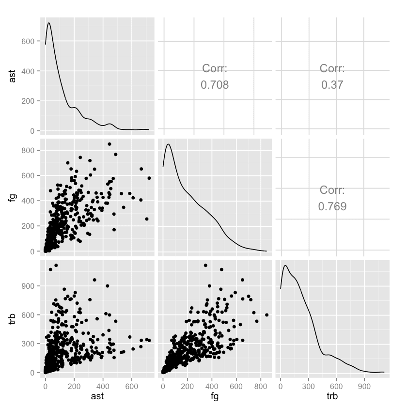
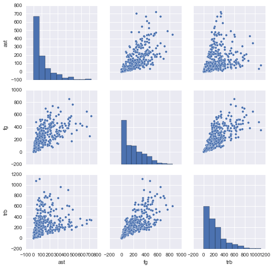
One common way to explore a data set is to see how different columns correlate to others. Let's compare the ast, fg, and trb columns.

R

library(GGally)
nba %>%
select(ast, fg, trb) %>%
ggpairs()

Python

import seaborn as sns
import matplotlib.pyplot as plt
sns.pairplot(nba[["ast", "fg", "trb"]])
plt.show()

In the end, both languages produce very similar plots. But in the code, we can see how the R data science ecosystem has many smaller packages (GGally is a helper package for ggplot2, the most-used R plotting package), and more visualization packages in general. 

In Python, matplotlib is the primary plotting package, and seaborn is a widely used layer over matplotlib.

With visualization in Python, there is generally one main way to do something, whereas in R, there are many packages supporting different methods of doing things (there are at least a half-dozen packages to make pair plots, for instance).

Again, neither approach is "better", but R may offer more flexibility just in terms of being able to pick and choose the package that works best for you.

Making Clusters of the Players

Another good way to explore this kind of data is to generate cluster plots. These will show which players are most similar.

(For now, we're just going to make the clusters; we'll plot them visually in the next step.)

R

library(cluster)
set.seed(1)
isGoodCol <- function(col){
  sum(is.na(col)) == 0 && is.numeric(col)
}
goodCols <- sapply(nba, isGoodCol)
clusters <- kmeans(nba[,goodCols], centers=5)
labels <- clusters$cluster

Python

from sklearn.cluster import KMeans
kmeans_model = KMeans(n_clusters=5, random_state=1)
good_columns = nba._get_numeric_data().dropna(axis=1)
kmeans_model.fit(good_columns)
labels = kmeans_model.labels_

In order to cluster properly, we need to remove any non-numeric columns and columns with missing values (NA, Nan, etc).

In R, we do this by applying a function across each column, and removing the column if it has any missing values or isn’t numeric. We then use the cluster package to perform k-means and find 5 clusters in our data. We set a random seed using set.seed to be able to reproduce our results.

In Python, we use the main Python machine learning package, scikit-learn, to fit a k-means clustering model and get our cluster labels. We perform very similar methods to prepare the data that we used in R, except we use the get_numeric_data and dropna methods to remove non-numeric columns and columns with missing values.

Plotting Players by Cluster

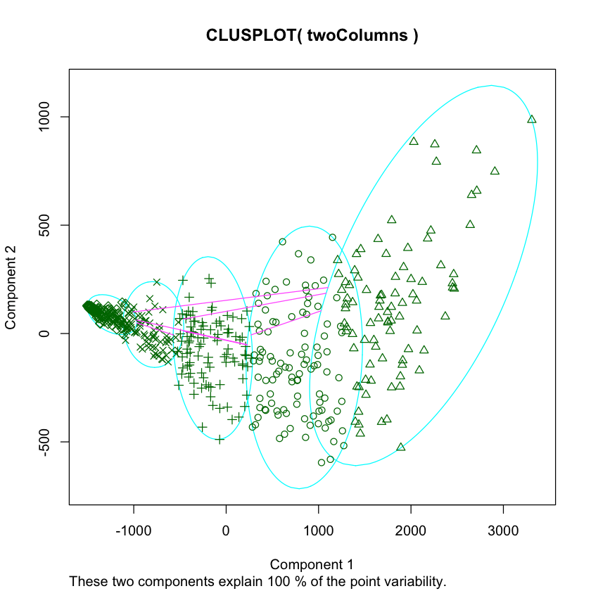
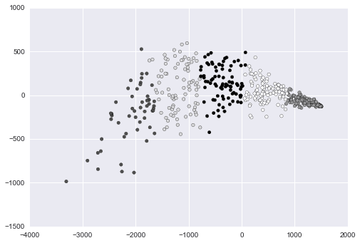
We can now plot out the players by cluster to discover patterns. One way to do this is to first use PCA to make our data  two-dimensional, then plot it, and shade each point according to cluster association.

R

nba2d <- prcomp(nba[,goodCols], center=TRUE)
twoColumns <- nba2d$x[,1:2]
clusplot(twoColumns, labels)

Python

from sklearn.decomposition import PCA
pca_2 = PCA(2)
plot_columns = pca_2.fit_transform(good_columns)
plt.scatter(x=plot_columns[:,0], y=plot_columns[:,1], c=labels)
plt.show()

Above, we made a scatter plot of our data, and shaded or changed the icon of each data point according to its cluster.

In R, we used the clusplot function, which is part of the cluster library. We performed PCA via the pccomp function that is built into R.

With Python, we used the PCA class in the scikit-learn library. We used matplotlib to create the plot.

Once again, we can see that while both languages take slightly different approaches, the final result and the amount of code required to get it is pretty similar.

Splitting Data into Training and Testing Sets

If we want to use R or Python for supervised machine learning, it’s a good idea to split the data into training and testing sets so we don’t overfit.

Let's compare how each language handles this common machine learning task:

R

trainRowCount <- floor(0.8 * nrow(nba))
set.seed(1)
trainIndex <- sample(1:nrow(nba), trainRowCount)
train <- nba[trainIndex,]
test <- nba[-trainIndex,]

Python

train = nba.sample(frac=0.8, random_state=1)
test = nba.loc[~nba.index.isin(train.index)]

Comparing Python vs R, we can see that R has more data analysis capability built-in, like floor, sample, and set.seed, whereas these in Python these are called via packages (math.floor, random.sample, random.seed).

In Python, a recent version of pandas came with a sample method that returns a certain proportion of rows randomly sampled from a source dataframe — this makes the code much more concise.

In R, there are packages to make sampling simpler, but they aren’t much more concise than using the built-in sample function. In both cases, we set a random seed to make the results reproducible.

R vs Python: Univariate Linear Regression

Continuing with common machine learning tasks, let’s say we want to predict number of assists per player from field goals made per player:

R

fit <- lm(ast ~ fg, data=train)
predictions <- predict(fit, test)

Python

from sklearn.linear_model import LinearRegression
lr = LinearRegression()
lr.fit(train[["fg"]], train["ast"])
predictions = lr.predict(test[["fg"]])

Python was a bit more concise in our previous step, but now R is more concise here!

Python's Scikit-learn package has a linear regression model that we can fit and generate predictions from. 

R relies on the built-in lm and predict functions. predict will behave differently depending on the kind of fitted model that is passed into it — it can be used with a variety of fitted models.

Calculating Summary Statistics for the Model

Another common machine learning task:

R

summary(fit)

Call:
lm(formula = ast ~ fg, data = train)
Residuals:Min 1Q Median 3Q Max
-228.26 -35.38 -11.45 11.99 559.61
[output truncated]

Python

import statsmodels.formula.api as sm
model = sm.ols(formula='ast ~ fga', data=train)
fitted = model.fit()
fitted.summary()

Dep. Variable: ast
R-squared: 0.568
Model: OLS
Adj. R-squared: 0.567
[output truncated]

As we can see above, we’ll need to do a bit more in Python than in R if we want to get summary statistics about the fit, like r-squared value.

With R, we can use the built-in summary function to get information on the model immediately. With Python, we need to use the statsmodels package, which enables many statistical methods to be used in Python.

We get similar results, although generally it’s a bit harder to do statistical analysis in Python, and some statistical methods that exist in R don’t exist in Python.

Fit a random forest model

Our linear regression worked well in the single variable case, but let's say we suspect there may be nonlinearities in the data. Thus, we want to fit a random forest model.

Here's how we might do that in each language:

R

library(randomForest)
predictorColumns <- c("age", "mp", "fg", "trb", "stl", "blk")
rf <- randomForest(train[predictorColumns], train$ast, ntree=100)
predictions <- predict(rf, test[predictorColumns])

Python

from sklearn.ensemble import RandomForestRegressor
predictor_columns = ["age", "mp", "fg", "trb", "stl", "blk"]
rf = RandomForestRegressor(n_estimators=100, min_samples_leaf=3)
rf.fit(train[predictor_columns], train["ast"])
predictions = rf.predict(test[predictor_columns])

The main difference here is that we needed to use the randomForest library in R to use the algorithm, whereas this is already built in to scikit-learn in Python.

Scikit-learn has a unified interface for working with many different machine learning algorithms in Python. There’s usually only one main implementation of each algorithm.

With R, there are many smaller packages containing individual algorithms, often with inconsistent ways to access them. This results in a greater diversity of algorithms (many have several implementations, and some are fresh out of research labs), but with a bit of a usability hit.

In other words, Python may be easier to use here, but R may be more flexible.

Calculating Error

Now that we’ve fit two models, let’s calculate error in R and Python. We’ll use MSE.

R

mean((test["ast"] - predictions)^2)

4573.86778567462

Python

from sklearn.metrics import mean_squared_error
mean_squared_error(test["ast"], predictions)

4166.9202475632374

In Python, the scikit-learn library has a variety of error metrics that we can use. In R, there are likely some smaller libraries that calculate MSE, but doing it manually is pretty easy in either language.

You may notice there’s a small difference in the results here — that's almost certainly due to parameter tuning, and isn’t a big deal.

(If you run this code on your own, you may also get slightly different numbers, depending on the versions of each package and language you're using).

R vs Python: Web Scraping, Part 1

We have data on NBA players from 2013-2014, but let’s web-scrape some additional data to supplement it.

We’ll just look at one box score from the NBA Finals here to save time.

R

library(RCurl)
url <- "http://www.basketball-reference.com/boxscores/201506140GSW.html"
data <- readLines(url)

Python

import requests
url = "http://www.basketball-reference.com/boxscores/201506140GSW.html"
data = requests.get(url).content

In Python, the requests package makes downloading web pages straightforward, with a consistent API for all request types. 

In R, RCurl provides a similarly simple way to make requests.

Both download the webpage to a character datatype.

Note: this step is unnecessary for the next step in R, but is shown for comparison’s sake.

Web Scraping, Part 2

Now that we have the web page dowloaded with both Python and R, we’ll need to parse it to extract scores for players.

R

library(rvest)
page <- read_html(url)
table <- html_nodes(page, ".stats_table")[3]
rows <- html_nodes(table, "tr")
cells <- html_nodes(rows, "td a")
teams <- html_text(cells)
extractRow <- function(rows, i){
  if(i == 1){
    return
  }
  row <- rows[i]
  tag <- "td"
  if(i == 2){
    tag <- "th"
  }
    items <- html_nodes(row, tag)
    html_text(items)
}
scrapeData <- function(team){
  teamData <- html_nodes(page, paste("#",team,"_basic", sep=""))
  rows <- html_nodes(teamData, "tr")
  lapply(seq_along(rows), extractRow, rows=rows)
}
data <- lapply(teams, scrapeData)

Python

from bs4 import BeautifulSoup
import re
soup = BeautifulSoup(data, 'html.parser')
box_scores = []
for tag in soup.find_all(id=re.compile("[A-Z]{3,}_basic")):
    rows = []
    for i, row in enumerate(tag.find_all("tr")):
        if i == 0:
        continue
    elif i == 1:
        tag = "th"
    else:
        tag = "td"
    row_data = [item.get_text() for item in row.find_all(tag)]
    rows.append(row_data)
    box_scores.append(rows)

In both languages, this code will create a list containing two lists

1. The box score for CLE
2. The box score for GSW
   

Both lists contain the headers, along with each player and their in-game stats. We won’t turn this into more training data now, but it could easily be transformed into a format that could be added to our nba dataframe.

The R code is more complex than the Python code, because there isn’t a convenient way to use regular expressions to select items, so we have to do additional parsing to get the team names from the HTML.

R also discourages using for loops in favor of applying functions along vectors. We use lapply to do this, but since we need to treat each row differently depending on whether it’s a header or not, we pass the index of the item we want, and the entire rows list into the function.

In R, we use rvest, a widely-used R web scraping package to extract the data we need. Note that we can pass a url directly into rvest, so the previous step wasn’t actually needed in R.

In Python, we use BeautifulSoup, the most commonly used web scraping package. It enables us to loop through the tags and construct a list of lists in a straightforward way.

R vs Python: Which is Better? It Depends!

We’ve now taken a look at how to analyze a data set with both R and Python. And as we can see, although they do things a little differently, both languages tend to require about the same amount of code to achieve the same output.

Of course, there are many tasks we didn’t dive into, such as persisting the results of our analysis, sharing the results with others, testing and making things production-ready, and making more visualizations.

There is a lot more to discuss on this topic, but just based on what we’ve done above, we can draw some meaningful conclusions about how the two differ.

(As far as which is actually better, that's a matter of personal preference.)

R is more functional, Python is more object-oriented.

As we saw from functions like lm, predict, and others, R lets functions do most of the work. Contrast this to the LinearRegression class in Python, and the sample method on Dataframes.

In terms of data analysis and data science, either approach works.

R has more data analysis functionality built-in, Python relies on packages.

When we looked at summary statistics, we could use the summary built-in function in R, but had to import the statsmodels package in Python. The Dataframe is a built-in construct in R, but must be imported via the pandas package in Python.

Python has “main” packages for data analysis tasks, R has a larger ecosystem of small packages.

With Python, we can do linear regression, random forests, and more with the scikit-learn package. It offers a consistent API, and is well-maintained.

In R, we have a greater diversity of packages, but also greater fragmentation and less consistency (linear regression is a built-in, lm, randomForest is a separate package, etc).

R has more statistical support in general.

R was built as a statistical language, and it shows. statsmodels in Python and other packages provide decent coverage for statistical methods, but the R ecosystem is far larger.

It’s usually more straightforward to do non-statistical tasks in Python.

With well-maintained libraries like BeautifulSoup and requests, web scraping in Python is more straightforward than in R.

This also applies to other tasks that we didn’t look into closely, like saving to databases, deploying web servers, or running complex workflows.

Since Python is used across a variety of industries and programming disciplines, it may be the better choice if you're combining your data work with other kinds of programming tasks. 

On the other hand, if you're focused on data and statistics, R offers some advantages due to its having been developed with a focus on statistics.

There are many parallels between the data analysis workflow in both.

There are clear points of similarity between both R and Python (pandas Dataframes were inspired by R dataframes, the rvest package was inspired by BeautifulSoup), and both ecosystems continue to grow stronger.

In fact, it’s remarkable how similar the syntax and approaches are for many common tasks in both languages.

R vs Python: Which Should You Learn?

At Dataquest, we’ve been best known for our Python courses, but we have totally reworked and relaunched our Data Analyst in R path because we feel R is another excellent language for data science.

We see both languages as complementary, and each language has its strengths and weaknesses. Either language could be used as your sole data analysis tool, as this walkthrough proves. Both languages have a lot of similarities in syntax and approach, and you can’t go wrong with either one.

Ultimately, you may end up wanting to learn Python and R so that you can make use of both languages’ strengths, choosing one or the other on a per-project basis depending on your needs.

And of course, knowing both also makes you a more flexible job candidate if you’re looking for a position in the data science world.

Vik Paruchuri

Vik is the CEO and Founder of Dataquest.

The post R vs Python for Data Analysis — An Objective Comparison appeared first on Dataquest.

from Planet Python
via read more