Stack Abuse: Deep Learning in Keras - Building a Deep Learning Model

Introduction

Deep learning is one of the most interesting and promising areas of artificial intelligence (AI) and machine learning currently. With great advances in technology and algorithms in recent years, deep learning has opened the door to a new era of AI applications.

In many of these applications, deep learning algorithms performed equal to human experts and sometimes surpassed them.

Python has become the go-to language for Machine Learning and many of the most popular and powerful deep learning libraries and frameworks like TensorFlow, Keras, and PyTorch are built in Python.

In this series, we'll be using Keras to perform Exploratory Data Analysis (EDA), Data Preprocessing and finally, build a Deep Learning Model and evaluate it.

In this stage, we will build a deep neural-network model that we will train and then use to predict house prices.

Defining the Model

A deep learning neural network is just a neural network with many hidden layers.

Defining the model can be broken down into a few characteristics:

• Number of Layers
• Types of these Layers
• Number of units (neurons) in each Layer
• Activation Functions of each Layer
• Input and output size

Deep Learning Layers

There are many types of layers for deep learning models. Convolutional and pooling layers are used in CNNs that classify images or do object detection, while recurrent layers are used in RNNs that are common in natural language processing and speech recognition.

We'll be using Dense and Dropout layers. Dense layers are the most common and popular type of layer - it's just a regular neural network layer where each of its neurons is connected to the neurons of the previous and next layer.

Each dense layer has an activation function that determines the output of its neurons based on the inputs and the weights of the synapses.

Dropout layers are just regularization layers that randomly drop some of the input units to 0. This helps in reducing the chance of overfitting the neural network.

Activation Functions

There are also many types of activation functions that can be applied to layers. Each of them links the neuron's input and weights in a different way and makes the network behave differently.

Really common functions are ReLU (Rectified Linear Unit), the Sigmoid function and the Linear function. We'll be mixing a couple of different functions.

Input and Output layers

In addition to hidden layers, models have an input layer and an output layer:

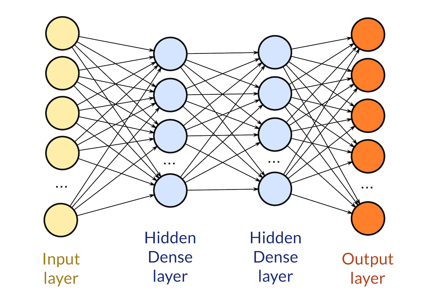
The number of neurons in the input layer is the same as the number of features in our data. We want to teach the network to react to these features. We have 67 features in the train_df and test_df dataframes - thus, our input layer will have 67 neurons. These will be the entry point of our data.

For the output layer - the number of neurons depends on your goal. Since we're just predicting the price - a single value, we'll use only one neuron. Classification models would have class-number of output neurons.

Since the output of the model will be a continuous number, we'll be using the linear activation function so none of the values get clipped.

Defining the Model Code

With these parameters in mind, let's define the model using Keras:

model = keras.Sequential([
    layers.Dense(64, activation='relu', input_shape=[train_df.shape[1]]),
    layers.Dropout(0.3, seed=2),
    layers.Dense(64, activation='swish'),
    layers.Dense(64, activation='relu'),
    layers.Dense(64, activation='swish'),
    layers.Dense(64, activation='relu'),
    layers.Dense(64, activation='swish'),
    layers.Dense(1)
])

Here, we've used Keras' Sequential() to instantiate a model. It takes a group of sequential layers and stacks them together into a single model. Into the Sequential() constructor, we pass a list that contains the layers we want to use in our model.

We've made several Dense layers and a single Dropout layer in this model. We've made the input_shape equal to the number of features in our data. We define that on the first layer as the input of that layer.

We've quickly dropped 30% of the input data to avoid overfitting. The seed is set to 2 so we get more reproducible results. If we just totally randomly dropped them, each model would be different.

Finally, we have a Dense layer with a single neuron as the output layer. By default, it has the linear activation function so we haven't set anything.

Compiling the Model

After defining our model, the next step is to compile it. Compiling a Keras model means configuring it for training.

To compile the model, we need to choose:

• The Loss Function -The lower the error, the closer the model is to the goal. Different problems require different loss functions to keep track of progress. Here's a list of supported loss functions.
• The Optimizer - The optimizing algorithm that helps us achieve better results for the loss function.
• Metrics - Metrics used to evaluate the model. For example, if we have a Mean Squared Error loss function, it would make sense to use the Mean Absolute Error as the metric used for evaluation.

With those in mind, let's compile the model:

optimizer = tf.keras.optimizers.RMSprop(learning_rate=0.001)

model.compile(loss=tf.keras.losses.MeanSquaredError(),
              optimizer=optimizer,
              metrics=['mae'])

Here, we've created an RMSprop optimizer, with a learning rate of 0.001. Feel free to experiment with other optimizers such as the Adam optimizer.

Note: You can either declare an optimizer and use that object or pass a string representation of it in the compile() method.

We've set the loss function to be Mean Squared Error. Again, feel free to experiment with other loss functions and evaluate the results. Since we have MSE as the loss function, we've opted for Mean Absolute Error as the metric to evaluate the model with.

Training the Model

After compiling the model, we can train it using our train_df dataset. This is done by fitting it via the fit() function:

history = model.fit(
    train_df, train_labels,
    epochs=70, validation_split=0.2
)

Here, we've passed the training data (train_df) and the train labels (train_labels).

Also, learning is an iterative process. We've told the network to go through this training dataset 70 times to learn as much as it can from it. The models' results in the last epoch will be better than in the first epoch.

Finally, we pass the training data that's used for validation. Specifically, we told it to use 0.2 (20%) of the training data to validate the results. Don't confuse this with the test_df dataset we'll be using to evaluate it.

The 20% will not be used for training, but rather for validation to make sure it makes progress.

This function will print the results of each epoch - the value of the loss function and the metric we've chosen to keep track of.

Once finished, we can take a look at how it's done through each epoch:

Epoch 65/70
59/59 [==============================] - 0s 2ms/step - loss: 983458944.0000 - mae: 19101.9668 - val_loss: 672429632.0000 - val_mae: 18233.3066
Epoch 66/70
59/59 [==============================] - 0s 2ms/step - loss: 925556032.0000 - mae: 18587.1133 - val_loss: 589675840.0000 - val_mae: 16720.8945
Epoch 67/70
59/59 [==============================] - 0s 2ms/step - loss: 1052588800.0000 - mae: 18792.9805 - val_loss: 608930944.0000 - val_mae: 16897.8262
Epoch 68/70
59/59 [==============================] - 0s 2ms/step - loss: 849525312.0000 - mae: 18392.6055 - val_loss: 613655296.0000 - val_mae: 16914.1777
Epoch 69/70
59/59 [==============================] - 0s 2ms/step - loss: 826159680.0000 - mae: 18177.8945 - val_loss: 588994816.0000 - val_mae: 16520.2832
Epoch 70/70
59/59 [==============================] - 0s 2ms/step - loss: 920209344.0000 - mae: 18098.7070 - val_loss: 571053952.0000 - val_mae: 16419.8359

After training, the model (stored in the model variable) will have learned what it can and is ready to make predictions. fit() also returns a dictionary that contains the loss function values and mae values after each epoch, so we can also make use of that. We've put that in the history variable.

Before making predictions, let's visualize how the loss value and mae changed over time:

model_history = pd.DataFrame(history.history)
model_history['epoch'] = history.epoch

fig, ax = plt.subplots(figsize=(14,8))
num_epochs = model_history.shape[0]
ax.plot(np.arange(0, num_epochs), model_history["mae"], 
        label="Training MAE", lw=3, color='#f4b400')
ax.plot(np.arange(0, num_epochs), model_history["val_mae"], 
        label="Validation MAE", lw=3, color='#0f9d58')
ax.legend()
plt.tight_layout()
plt.show()

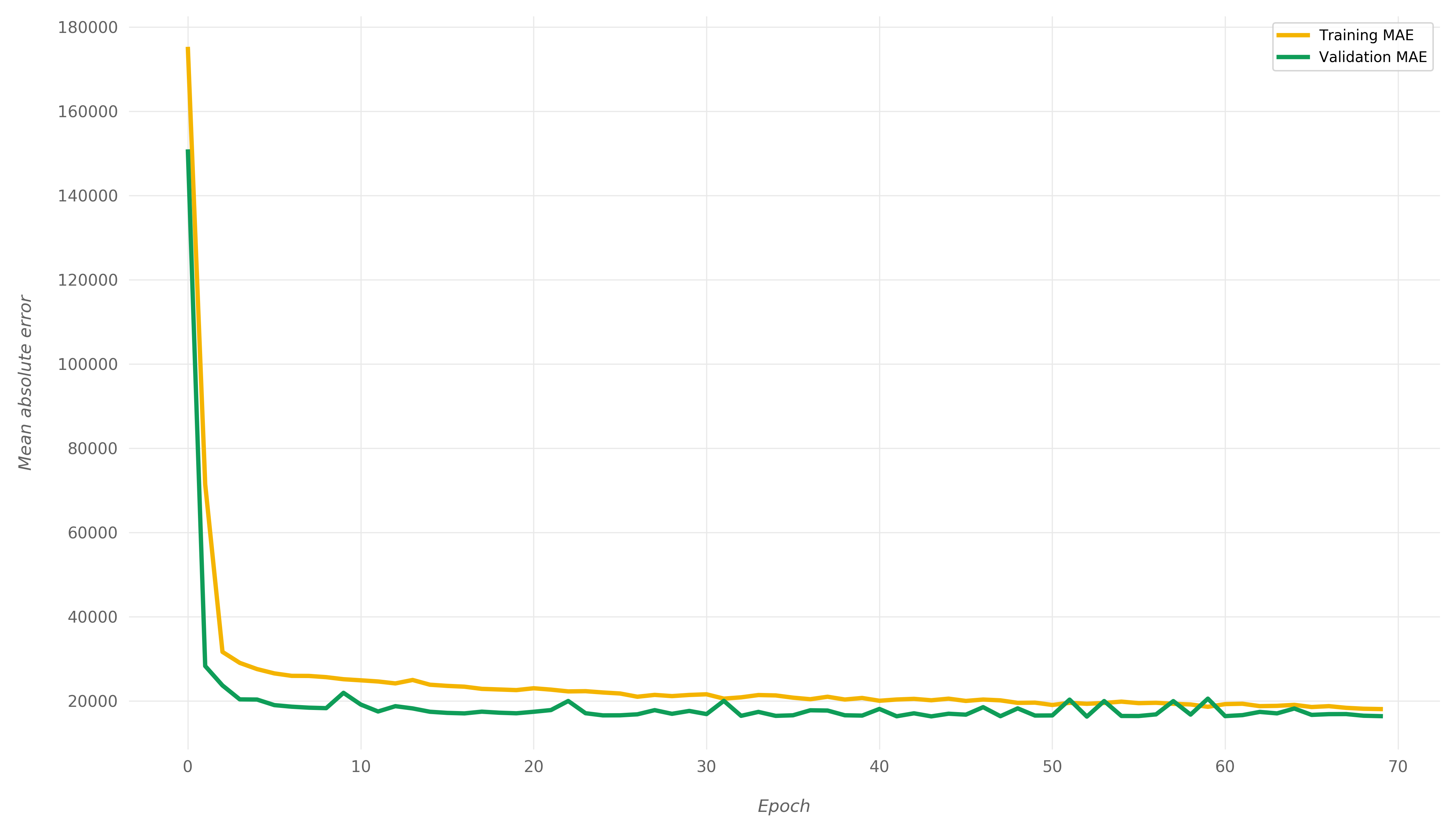
We can clearly see both the mae and loss values go down over time. This is exactly what we want - the model got more accurate with the predictions over time.

Making Predictions with the Model

Now that our model is trained, let's use it to make some predictions. We take an item from the test data (in test_df):

test_unit = test_df.iloc[[0]]

This item stored in test_unit has the following values, cropped at only 7 entries for brevity:

	Lot Frontage	Lot Area	Overall Qual	Overall Cond	Year Built	Total Bsmt SF	1st Flr SF
14	0.0157117	-0.446066	1.36581	-0.50805	0.465714	1.01855	0.91085

These are the values of the feature unit and we'll use the model to predict its sale price:

test_pred = model.predict(test_unit).squeeze()

We used the predict() function of our model, and passed the test_unit into it to make a prediction of the target variable - the sale price.

Note: predict() returns a NumPy array so we used squeeze(), which is a NumPy function to "squeeze" this array and get the prediction value out of it as a number, not an array.

Now, let's get the actual price of the unit from test_labels:

test_lbl = test_labels.iloc[0]

And now, let's compare the predicted price and the actual price:

print("Model prediction = {:.2f}".format(test_pred))
print("Actual value = {:.2f}".format(test_lbl))

Model prediction = 225694.92
Actual value = 212000.00

So the actual sale price for this unit is $212,000 and our model predicted it to be ​*$225,694*. That's fairly close, though the model overshot the price ~5%.

Let's try another unit from test_df:

test_unit = test_df.iloc[[100]]

And we'll repeat the same process to compare the prices:

test_pred = model.predict(test_unit).squeeze()
test_lbl = test_labels.iloc[100]
print("Model prediction = {:.2f}".format(test_pred))
print("Actual value = {:.2f}".format(test_lbl))

Model prediction = 330350.47
Actual value = 340000.00

So for this unit, the actual price is $340,000 and the predicted price is ​*$330,350*. Again, not quite on point, but it's an error of just ~3%. That's very accurate.

Evaluating the Model

This is the final stage in our journey of building a Keras deep learning model. In this stage we will use the model to generate predictions on all the units in our testing data (test_df) and then calculate the mean absolute error of these predictions by comparing them to the actual true values (test_labels).

Keras provides the evaluate() function which we can use with our model to evaluate it. evaluate() calculates the loss value and the values of all metrics we chose when we compiled the model.

We chose MAE to be our metric because it can be easily interpreted. MAE value represents the average value of model error:
$$
\begin{equation*}
\text{MAE}(y, \hat{y}) = \frac{1}{n} \sum_{i=1}^{n} \left| y_i - \hat{y}_i \right|.
\end{equation*}
$$

For our convenience, the evaluate() function takes care of this for us:

loss, mae = model.evaluate(test_df, test_labels, verbose=0)

To this method, we pass the test data for our model (to be evaluated upon) and the actual data (to be compared to). Furthermore, we've used the verbose argument to avoid printing any additional data that's not really needed.

Let's run the code and see how it does:

print('MAE = {:.2f}'.format(mae))

MAE = 17239.13

The mean absolute error is 17239.13. That's to say, for all units, the model on average predicted $17,239 above or below the actual price.

Interpretation of Model Performance

How good is that result? If we look back at the EDA we have done on SalePrice, we can see that the average sale price for the units in our original data is $180,796. That said, a MAE of 17,239 is fairly good.

To interpret these results in another way, let's plot the predictions against the actual prices:

test_predictions_ = model.predict(test_df).flatten()
test_labels_ = test_labels.to_numpy().flatten()
fig, ax = plt.subplots(figsize=(14,8))
plt.scatter(test_labels_, test_predictions_, alpha=0.6, 
            color='#ff7043', lw=1, ec='black')
lims = [0, max(test_predictions_.max(), test_labels_.max())]
plt.plot(lims, lims, lw=1, color='#00acc1')
plt.tight_layout()
plt.show()

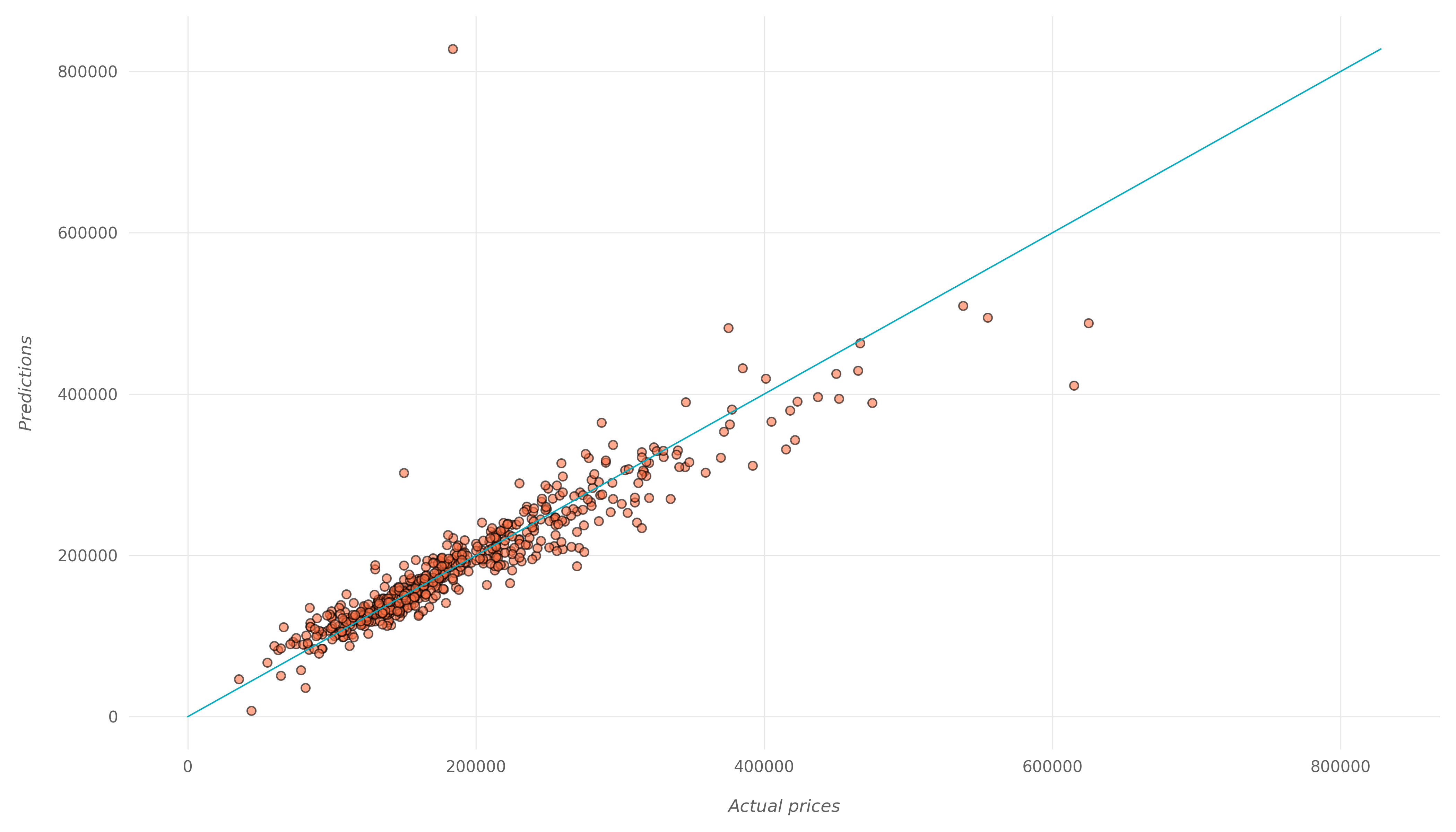
If our model was 100% accurate with 0 MAE, all points would appear exactly on the diagonal cyan line. However, no model is 100% accurate, and we can see that most points are close to the diagonal line which means the predictions are close to the actual values.

There are a few outliers, some of which are off by a lot. These bring the average MAE of our model up drastically. In reality, for most of these points, the MAE is much less than 17,239.

We can inspect these points and find out if we can perform some more data preprocessing and feature engineering to make the model predict them more accurately.

Conclusion

In this tutorial, we've built a deep learning model using Keras, compiled it, fitted it with the clean data we've prepared and finally - performed predictions based on what it's learned.

While not 100% accurate, we managed to get some very decent results with a small number of outliers.

from Planet Python
via read more