John Cook: Solving Van der Pol equation with ivp_solve

Van der Pol’s differential equation is

The equation describes a system with nonlinear damping, the degree of damping given by μ. If μ = 0 the system is linear and undamped, but for positive μ the system is nonlinear and damped. We will plot the phase portrait for the solution to Van der Pol’s equation in Python using SciPy’s new ODE solver ivp_solve.

The function ivp_solve does not solve second-order systems of equations directly. It solves systems of first-order equations, but a second-order differential equation can be recast as a pair of first-order equations by introducing the first derivative as a new variable.

Since y is the derivative of x, the phase portrait is just the plot of (x, y).

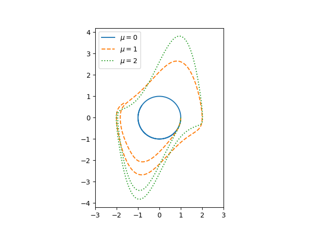
If μ = 0, we have a simple harmonic oscillator and the phase portrait is simply a circle. For larger values of μ the solutions enter limiting cycles, but the cycles are more complicated than just circles.

Here’s the Python code that made the plot.

from scipy import linspace
from scipy.integrate import solve_ivp
import matplotlib.pyplot as plt

def vdp(t, z):
    x, y = z
    return [y, mu*(1 - x**2)*y - x]

a, b = 0, 10

mus = [0, 1, 2]
styles = ["-", "--", ":"]
t = linspace(a, b, 1000)

for mu, style in zip(mus, styles):
    sol = solve_ivp(vdp, [a, b], [1, 0], t_eval=t)
    plt.plot(sol.y[0], sol.y[1], style)
  
# make a little extra horizontal room for legend
plt.xlim([-3,3])    
plt.legend([f"$\mu={m}$" for m in mus])
plt.axes().set_aspect(1)

Related posts

• Duffing equation
• The other butterfly effect
• Linear mechanical vibrations

from Planet Python
via read more