Introduction
This article is inspired by a tweet from Peter Baumgartner. In the tweet he mentioned the Fisher-Jenks algorithm and showed a simple example of ranking data into natural breaks using the algorithm. Since I had never heard about it before, I did some research.
After learning more about it, I realized that it is very complimentary to my previous article on Binning Data and it is intuitive and easy to use in standard pandas analysis. It is definitely an approach I would have used in the past if I had known it existed.
I suspect many people are like me and have never heard of the concept of natural breaks before but have probably done something similar on their own data. I hope this article will expose this simple and useful approach to others so that they can add it to their python toolbox.
The rest of this article will discuss what the Jenks optimization method (or Fisher-Jenks algorithm) is and how it can be used as a simple tool to cluster data using “natural breaks”.
Background
Thanks again to Peter Baumgartner for this tweet which piqued my interest.
Randomly helpful data thing: need to cluster in 1D? Try the Fisher-Jenks algorithm!
— Peter Baumgartner (@pmbaumgartner) December 13, 2019
Here's how I use it: I if want to select the top-n things, but I'm not sure what n should be, this can give an data-determined n. pic.twitter.com/rkM8w3aikk
This algorithm was originally designed as a way to make chloropleth maps more visually representative of the underlying data. This approach certainly works for maps but I think it is also useful for other applications. This method can be used in much the same way that simple binning of data might be used to group numbers together.
What we are trying to do is identify natural groupings of numbers that are “close” together while also maximizing the distance between the other groupings. Fisher developed a clustering algorithm that does this with 1 dimensional data (essentially a single list of numbers). In many ways it is similar to k-means clustering but is ultimately a simpler and faster algorithm because it only works on 1 dimensional data. Like k-means, you do need to specify the number of clusters. Therefore domain knowledge and understanding of the data are still essential to using this effectively.
The algorithm uses an iterative approach to find the best groupings of numbers based on how close they are together (based on variance from the group’s mean) while also trying to ensure the different groupings are as distinct as possible (by maximizing the group’s variance between groups). I found this page really useful to understanding some of the history of the algorithm and this article goes into more depth behind the math of the approach.
Regardless of the math, the concept is very similar to how you would intuitively break groups of numbers. For example, let’s look at some sample sales numbers for 9 accounts. Given the data below, if you were asked to break the accounts into 2 buckets, based solely on sales, you would likely do something like this:
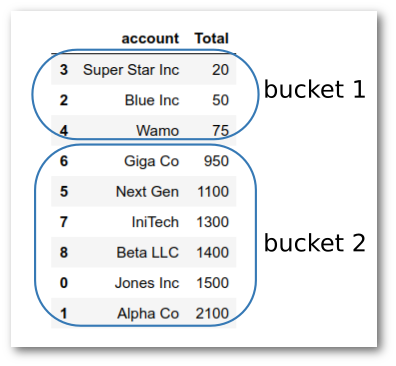
Without knowing the actual details of the algorithm, you would have known that 20, 50 and 75 are all pretty close to each other. Then, there is a big gap between 75 and 950 so that would be a “natural break” that you would utilize to bucket the rest of your accounts.
This is exactly what the Jenks optimization algorithm does. It uses an iterative approach to identify the “natural breaks” in the data.
What I find especially appealing about this algorithm is that the breaks are meant to be intuitive. It is relatively easy to explain to business users how these groupings were developed.
Before I go any further, I do want to make clear that in my research, I found this approach referred to by the following names: “Jenks Natural Breaks”, “Fisher-Jenks optimization”, “Jenks natural breaks optimization”, “Jenks natural breaks classification method”, “Fisher-Jenks algorithm” and likely some others. I mean no disrespect to anyone involved but for the sake of simplicity I will use the term Jenks optimization or natural breaks as a generic description of the method going forward.
Implementation
For the purposes of this article, I will use jenkspy from Matthieu Viry. This specific implementation appears to be actively maintained and has a compiled c component to ensure fast implementation. The algorithm is relatively simple so there are other approaches out there but as of this writing, this one seems to be the best I can find.
On my system, the install with conda install -c conda-forge jenkspy worked seamlessly. You can follow along in this notebook if you want to.
We can get started with a simple data set to clearly illustrate finding natural breaks in the data and how it compares to other binning approaches discussed in the past.
First, we import the modules and load the sample data:
import pandas as pd
import jenkspy
sales = {
'account': [
'Jones Inc', 'Alpha Co', 'Blue Inc', 'Super Star Inc', 'Wamo',
'Next Gen', 'Giga Co', 'IniTech', 'Beta LLC'
],
'Total': [1500, 2100, 50, 20, 75, 1100, 950, 1300, 1400]
}
df = pd.DataFrame(sales)
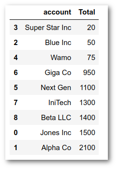
df.sort_values(by='Total')
Which yields the DataFrame:
In order to illustrate how natural breaks are found, we can start by contrasting it with how quantiles are determined. For example, what happens if we try to use pd.qcut with 2 quantiles? Will that give us a similar result?
df['quantile'] = pd.qcut(df['Total'], q=2, labels=['bucket_1', 'bucket_2'])
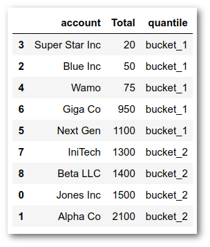
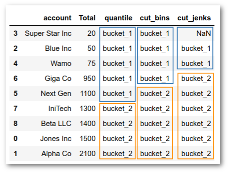
As you can see this approach tries to find two equal distribution of the numbers. The result is that bucket_1 covers the values from 20 - 1100 and bucket_2 includes the rest.
This does not feel like where we would like to have the break if we were seeking to explain a grouping in a business setting. If the question was something like “How do we divide our customers into Top and and Bottom customer segment groups?”
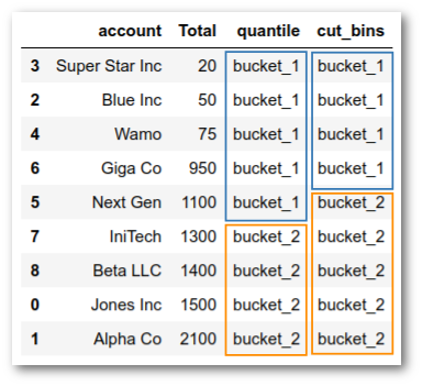
We can also use pd.cut to create two buckets:
df['cut_bins'] = pd.cut(df['Total'],
                        bins=2,
                        labels=['bucket_1', 'bucket_2'])
Which gets us closer but still not quite where we would ideally like to be:
If we want to find the natural breaks using jenks_breaks , we need to pass the column of data and the number of clusters we want, then the function will give us a simple list with our boundaries:
breaks = jenkspy.jenks_breaks(df['Total'], nb_class=2)
print(breaks)
[20.0, 75.0, 2100.0]
As I discussed in the previous article, we can pass these boundaries to cut and assign back to our DataFrame for more analysis:
df['cut_jenks'] = pd.cut(df['Total'],
                        bins=breaks,
                        labels=['bucket_1', 'bucket_2'])
We are almost there, except for the pesky NaN in the first row:
The easiest approach to fix the NaN is to use the include_lowest=True parameter to make sure that the lowest value in the data is included:
df['cut_jenksv2'] = pd.cut(df['Total'],
                        bins=breaks,
                        labels=['bucket_1', 'bucket_2'],
                        include_lowest=True)
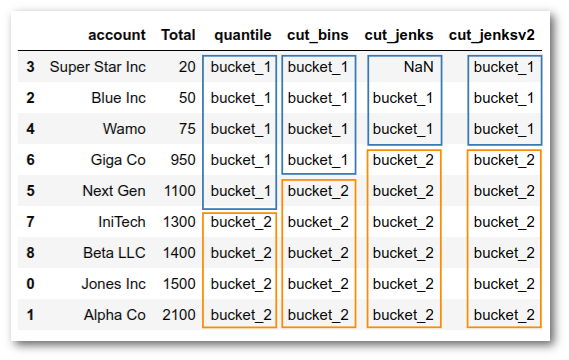
Now, we have the buckets set up like our intuition would expect.
I think you will agree that the process of determining the natural breaks was pretty straightforward and easy to use when combined with pd.cut.
Just to get one more example, we can see what 4 buckets would look like with natural breaks and with a quantile cut approach:
df['quantilev2'] = pd.qcut(
    df['Total'], q=4, labels=['bucket_1', 'bucket_2', 'bucket_3', 'bucket_4'])

df['cut_jenksv3'] = pd.cut(
    df['Total'],
    bins=jenkspy.jenks_breaks(df['Total'], nb_class=4),
    labels=['bucket_1', 'bucket_2', 'bucket_3', 'bucket_4'],
    include_lowest=True)

df.sort_values(by='Total')
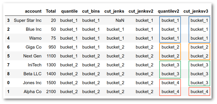
By experimenting with different numbers of groups, you can get a feel for how natural breaks behave differently than the quantile approach we may normally use. In most cases, you will need to rely on your business knowledge to determine which approach makes most sense and how many groups to create.
Summary
The simple example in this article illustrates how to use Jenks optimization to find natural breaks in your numeric data. For these examples, you could easily calculate the breaks by hand or by visually inspecting the data. However, once your data grows to thousands or millions of rows, that approach is impractical.
As a small side note, if you want to make yourself feel good about using python, take a look at what it takes to implement something similar in Excel. Painful, to say the least.
What is exciting about this technique is that it is very easy to incorporate into your data analysis process and provides a simple technique to look at grouping or clustering your data that can be intuitively obvious to your business stakeholders. It is certainly no substitution for a true customer segmentation approach where you might use a scikit-learn clustering algorithm. However it is a handy option to have available as you start exploring your data and eventually evolve into more sophisticated clustering approaches.
credit: Photo by Alice Pasqual
from Planet Python
via read more


No comments:
Post a Comment