Computer vision is an exciting and growing field. There are tons of interesting problems to solve! One of them is face detection: the ability of a computer to recognize that a photograph contains a human face, and tell you where it is located. In this article, you’ll learn about face detection with Python.
To detect any object in an image, it is necessary to understand how images are represented inside a computer, and how that objects differs visually from any other object.
Once that is done, the process of scanning an image and looking for those visual cues needs to be automated and optimized. All these steps come together to form a fast and reliable computer vision algorithm.
In this tutorial you’ll learn:
- What face detection is
- How computers understand features in images
- How to quickly analyze many different features to reach a decision
- How to use a minimal Python solution for detecting human faces in images
What Is Face Detection?
Face detection is a type of computer vision technology that is able to identify people’s faces within digital images. This is very easy for humans, but computers need precise instructions. The images might contain many objects that aren’t human faces, like buildings, cars, animals, and so on.
It is distinct from other computer vision technologies that involve human faces, like facial recognition, analysis, and tracking.
Facial recognition involves identifying the face in the image as belonging to person X and not person Y. It is often used for biometric purposes, like unlocking your smartphone.
Facial analysis tries to understand something about people from their facial features, like determining their age, gender, or the emotion they are displaying.
Facial tracking is mostly present in video analysis and tries to follow a face and its features (eyes, nose, and lips) from frame to frame. The most popular applications are various filters available in mobile apps like Snapchat.
All of these problems have different technological solutions. This tutorial will focus on a traditional solution for the first challenge: face detection.
How Do Computers “See” Images?
The smallest element of an image is called a pixel, or a picture element. It is basically a dot in the picture. An image contains multiple pixels arranged in rows and columns.
You will often see the number of rows and columns expressed as the image resolution. For example, an Ultra HD TV has the resolution of 3840x2160, meaning it is 3840 pixels wide and 2160 pixels high.
But a computer does not understand pixels as dots of color. It only understands numbers. To convert colors to numbers, the computer uses various color models.
In color images, pixels are often represented in the RGB color model. RGB stands for Red Green Blue. Each pixel is a mix of those three colors. RGB is great at modeling all the colors humans perceive by combining various amounts of red, green, and blue.
Since a computer only understand numbers, every pixel is represented by three numbers, corresponding to the amounts of red, green, and blue present in that pixel. You can learn more about color spaces in Image Segmentation Using Color Spaces in OpenCV + Python.
In grayscale (black and white) images, each pixel is a single number, representing the amount of light, or intensity, it carries. In many applications, the range of intensities is from 0 (black) to 255 (white). Everything between 0 and 255 is various shades of gray.
If each grayscale pixel is a number, an image is nothing more than a matrix (or table) of numbers:

Example 3x3 image with pixel values and colors
In color images, there are three such matrices representing the red, green, and blue channels.
What Are Features?
A feature is a piece of information in an image that is relevant to solving a certain problem. It could be something as simple as a single pixel value, or more complex like edges, corners, and shapes. You can combine multiple simple features into a complex feature.
Applying certain operations to an image produces information that could be considered features as well. Computer vision and image processing have a large collection of useful features and feature extracting operations.
Basically, any inherent or derived property of an image could be used as a feature to solve tasks.
Preparation
To run the code examples, you need to set up an environment with all the necessary libraries installed. The simplest way is to use conda.
You will need three libraries:
scikit-imagescikit-learnopencv
To create an environment in conda, run these commands in your shell:
$ conda create --name face-detection python=3.7
$ source activate face-detection
(face-detection)$ conda install scikit-learn
(face-detection)$ conda install -c conda-forge scikit-image
(face-detection)$ conda install -c menpo opencv3
If you are having problems installing OpenCV correctly and running the examples, try consulting their Installation Guide or the article on OpenCV Tutorials, Resources, and Guides.
Now you have all the packages necessary to practice what you learn in this tutorial.
Viola-Jones Object Detection Framework
This algorithm is named after two computer vision researchers who proposed the method in 2001: Paul Viola and Michael Jones.
They developed a general object detection framework that was able to provide competitive object detection rates in real time. It can be used to solve a variety of detection problems, but the main motivation comes from face detection.
The Viola-Jones algorithm has 4 main steps, and you’ll learn more about each of them in the sections that follow:
- Selecting Haar-like features
- Creating an integral image
- Running AdaBoost training
- Creating classifier cascades
Given an image, the algorithm looks at many smaller subregions and tries to find a face by looking for specific features in each subregion. It needs to check many different positions and scales because an image can contain many faces of various sizes. Viola and Jones used Haar-like features to detect faces.
Haar-Like Features
All human faces share some similarities. If you look at a photograph showing a person’s face, you will see, for example, that the eye region is darker than the bridge of the nose. The cheeks are also brighter than the eye region. We can use these properties to help us understand if an image contains a human face.
A simple way to find out which region is lighter or darker is to sum up the pixel values of both regions and comparing them. The sum of pixel values in the darker region will be smaller than the sum of pixels in the lighter region. This can be accomplished using Haar-like features.
A Haar-like feature is represented by taking a rectangular part of an image and dividing that rectangle into multiple parts. They are often visualized as black and white adjacent rectangles:

Basic Haar-like rectangle features
In this image, you can see 4 basic types of Haar-like features:
- Horizontal feature with two rectangles
- Vertical feature with two rectangles
- Vertical feature with three rectangles
- Diagonal feature with four rectangles
The first two examples are useful for detecting edges. The third one detects lines, and the fourth one is good for finding diagonal features. But how do they work?
The value of the feature is calculated as a single number: the sum of pixel values in the black area minus the sum of pixel values in the white area. For uniform areas like a wall, this number would be close to zero and won’t give you any meaningful information.
To be useful, a Haar-like feature needs to give you a large number, meaning that the areas in the black and white rectangles are very different. There are known features that perform very well to detect human faces:

Haar-like feature applied on the eye region. (Image:
Wikipedia)
In this example, the eye region is darker than the region below. You can use this property to find which areas of an image give a strong response (large number) for a specific feature:

Haar-like feature applied on the bridge of the nose. (Image:
Wikipedia)
This example gives a strong response when applied to the bridge of the nose. You can combine many of these features to understand if an image region contains a human face.
As mentioned, the Viola-Jones algorithm calculates a lot of these features in many subregions of an image. This quickly becomes computationally expensive: it takes a lot of time using the limited resources of a computer.
To tackle this problem, Viola and Jones used integral images.
Integral Images
An integral image (also known as a summed-area table) is the name of both a data structure and an algorithm used to obtain this data structure. It is used as a quick and efficient way to calculate the sum of pixel values in an image or rectangular part of an image.
In an integral image, the value of each point is the sum of all pixels above and to the left, including the target pixel:
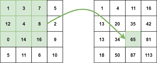
Calculating an integral image from pixel values
The integral image can be calculated in a single pass over the original image. This reduces summing the pixel intensities within a rectangle into only three operations with four numbers, regardless of rectangle size:
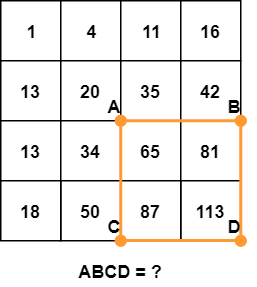
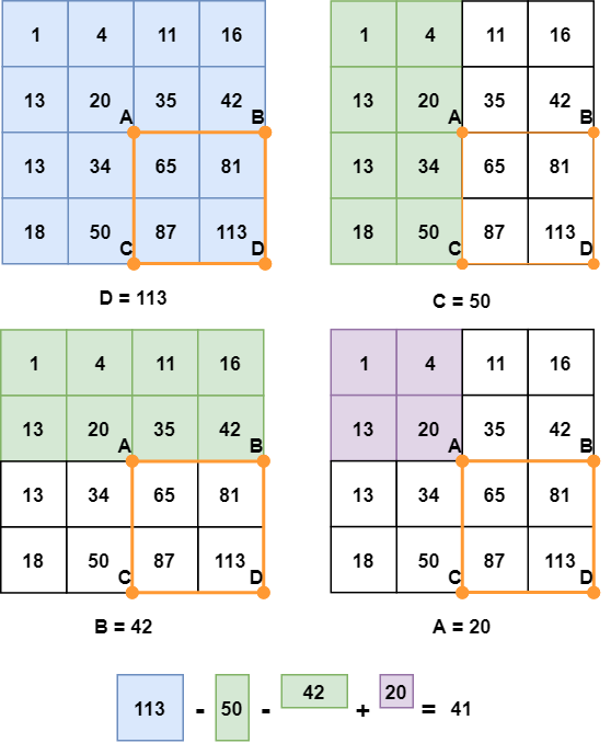
Calculate the sum of pixels in the orange rectangle.
The sum of pixels in the rectangle ABCD can be derived from the values of points A, B, C, and D, using the formula D - B - C + A. It is easier to understand this formula visually:
Calculating the sum of pixels step by step
You’ll notice that subtracting both B and C means that the area defined with A has been subtracted twice, so we need to add it back again.
Now you have a simple way to calculate the difference between the sums of pixel values of two rectangles. This is perfect for Haar-like features!
But how do you decide which of these features and in what sizes to use for finding faces in images? This is solved by a machine learning algorithm called boosting. Specifically, you will learn about AdaBoost, short for Adaptive Boosting.
AdaBoost
Boosting is based on the following question: “Can a set of weak learners create a single strong learner?” A weak learner (or weak classifier) is defined as a classifier that is only slightly better than random guessing.
In face detection, this means that a weak learner can classify a subregion of an image as a face or not-face only slightly better than random guessing. A strong learner is substantially better at picking faces from non-faces.
The power of boosting comes from combining many (thousands) of weak classifiers into a single strong classifier. In the Viola-Jones algorithm, each Haar-like feature represents a weak learner. To decide the type and size of a feature that goes into the final classifier, AdaBoost checks the performance of all classifiers that you supply to it.
To calculate the performance of a classifier, you evaluate it on all subregions of all the images used for training. Some subregions will produce a strong response in the classifier. Those will be classified as positives, meaning the classifier thinks it contains a human face.
Subregions that don’t produce a strong response don’t contain a human face, in the classifiers opinion. They will be classified as negatives.
The classifiers that performed well are given higher importance or weight. The final result is a strong classifier, also called a boosted classifier, that contains the best performing weak classifiers.
The algorithm is called adaptive because, as training progresses, it gives more emphasis on those images that were incorrectly classified. The weak classifiers that perform better on these hard examples are weighted more strongly than others.
Let’s look at an example:
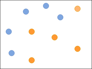
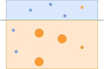
The blue and orange circles are samples that belong to different categories.
Imagine that you are supposed to classify blue and orange circles in the following image using a set of weak classifiers:
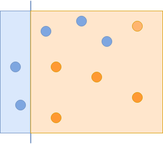
The first weak classifier classifies some of the blue circles correctly.
The first classifier you use captures some of the blue circles but misses the others. In the next iteration, you give more importance to the missed examples:
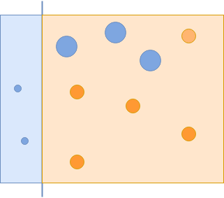
The missed blue samples are given more importance, indicated by size.
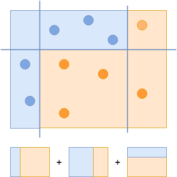
The second classifier that manages to correctly classify those examples will get a higher weight. Remember, if a weak classifier performs better, it will get a higher weight and thus higher chances to be included in the final, strong classifiers:
The second classifier captures the bigger blue circles.
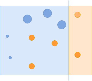
Now you have managed to capture all of the blue circles, but incorrectly captured some of the orange circles. These incorrectly classified orange circles are given more importance in the next iteration:
The misclassified orange circles are given more importance, and others are reduced.
The final classifier manages to capture those orange circles correctly:
The third classifier captures the remaining orange circles.
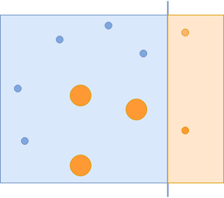
To create a strong classifier, you combine all three classifiers to correctly classify all examples:
The final, strong classifier combines all three weak classifiers.
Using a variation of this process, Viola and Jones have evaluated hundreds of thousands of classifiers that specialize in finding faces in images. But it would be computationally expensive to run all these classifiers on every region in every image, so they created something called a classifier cascade.
Cascading Classifiers
The definition of a cascade is a series of waterfalls coming one after another. A similar concept is used in computer science to solve a complex problem with simple units. The problem here is reducing the number of computations for each image.
To solve it, Viola and Jones turned their strong classifier (consisting of thousands of weak classifiers) into a cascade where each weak classifier represents one stage. The job of the cascade is to quickly discard non-faces and avoid wasting precious time and computations.
When an image subregion enters the cascade, it is evaluated by the first stage. If that stage evaluates the subregion as positive, meaning that it thinks it’s a face, the output of the stage is maybe.
If a subregion gets a maybe, it is sent to the next stage of the cascade. If that one gives a positive evaluation, then that’s another maybe, and the image is sent to the third stage:
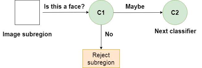
A weak classifier in a cascade
This process is repeated until the image passes through all stages of the cascade. If all classifiers approve the image, it is finally classified as a human face and is presented to the user as a detection.
If, however, the first stage gives a negative evaluation, then the image is immediately discarded as not containing a human face. If it passes the first stage but fails the second stage, it is discarded as well. Basically, the image can get discarded at any stage of the classifier:
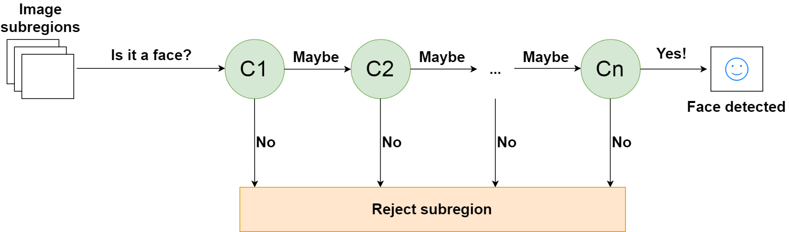
A cascade of _n_ classifiers for face detection
This is designed so that non-faces get discarded very quickly, which saves a lot of time and computational resources. Since every classifier represents a feature of a human face, a positive detection basically says, “Yes, this subregion contains all the features of a human face.” But as soon as one feature is missing, it rejects the whole subregion.
To accomplish this effectively, it is important to put your best performing classifiers early in the cascade. In the Viola-Jones algorithm, the eyes and nose bridge classifiers are examples of best performing weak classifiers.
Now that you understand how the algorithm works, it is time to use it to detect faces with Python.
Using a Viola-Jones Classifier
Training a Viola-Jones classifier from scratch can take a long time. Fortunately, a pre-trained Viola-Jones classifier comes out-of-the-box with OpenCV! You will use that one to see the algorithm in action.
First, find and download an image that you would like to scan for the presence of human faces. Here’s an example:

Example stock photo for face detection (
Image source)
Import OpenCV and load the image into memory:
import cv2 as cv

# Read image from your local file system
original_image = cv.imread('path/to/your-image.jpg')

# Convert color image to grayscale for Viola-Jones
grayscale_image = cv.cvtColor(original_image, cv.COLOR_BGR2GRAY)
Next, you need to load the Viola-Jones classifier. If you installed OpenCV from source, it will be in the folder where you installed the OpenCV library.
Depending on the version, the exact path might vary, but the folder name will be haarcascades, and it will contain multiple files. The one you need is called haarcascade_frontalface_alt.xml.
If for some reason, your installation of OpenCV did not get the pre-trained classifier, you can obtain it from the OpenCV GitHub repo:
# Load the classifier and create a cascade object for face detection
face_cascade = cv.CascadeClassifier('path/to/haarcascade_frontalface_alt.xml')
The face_cascade object has a method detectMultiScale(), which receives an image as an argument and runs the classifier cascade over the image. The term MultiScale indicates that the algorithm looks at subregions of the image in multiple scales, to detect faces of varying sizes:
detected_faces = face_cascade.detectMultiScale(grayscale_image)
The variable detected_faces now contains all the detections for the target image. To visualize the detections, you need to iterate over all detections and draw rectangles over the detected faces.
OpenCV’s rectangle() draws rectangles over images, and it needs to know the pixel coordinates of the top-left and bottom-right corner. The coordinates indicate the row and column of pixels in the image.
Luckily, detections are saved as pixel coordinates. Each detection is defined by its top-left corner coordinates and width and height of the rectangle that encompasses the detected face.
Adding the width to the row and height to the column will give you the bottom-right corner of the image:
for (column, row, width, height) in detected_faces:
    cv.rectangle(
        original_image,
        (column, row),
        (column + width, row + height),
        (0, 255, 0),
        2
    )
rectangle() accepts the following arguments:
- The original image
- The coordinates of the top-left point of the detection
- The coordinates of the bottom-right point of the detection
- The color of the rectangle (a tuple that defines the amount of red, green, and blue (
0-255))
- The thickness of the rectangle lines
Finally, you need to display the image:
cv.imshow('Image', original_image)
cv.waitKey(0)
cv.destroyAllWindows()
imshow() displays the image. waitKey() waits for a keystroke. Otherwise, imshow() would display the image and immediately close the window. Passing 0 as the argument tells it to wait indefinitely. Finally, destroyAllWindows() closes the window when you press a key.
Here’s the result:
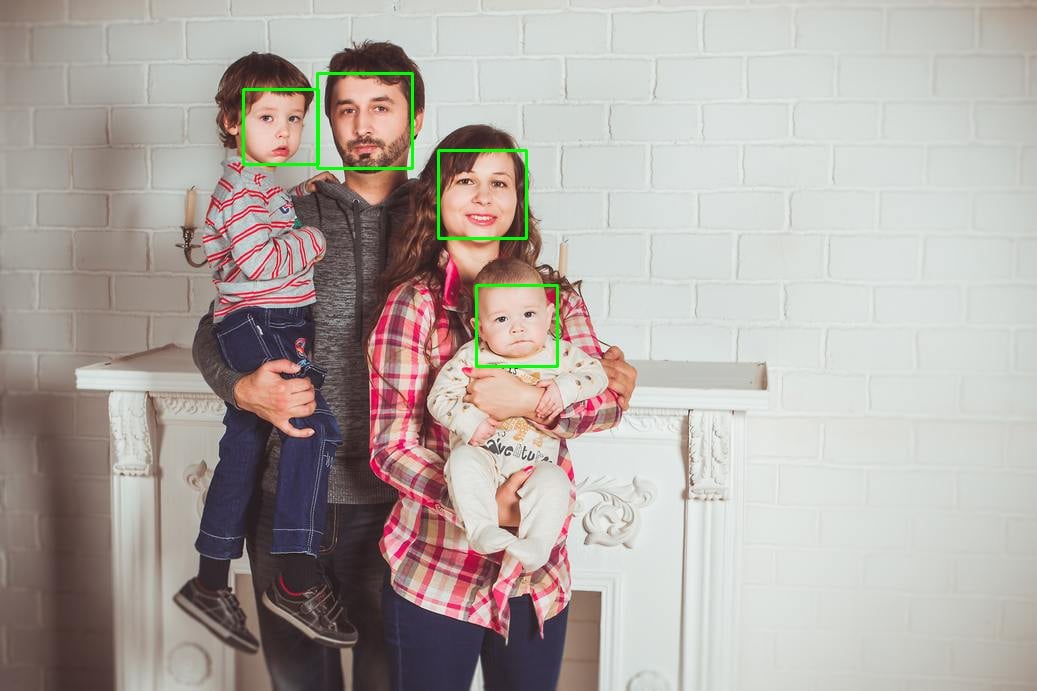
Original image with detections
That’s it! You now have a ready-to-use face detector in Python.
If you really want to train the classifier yourself, scikit-image offers a tutorial with the accompanying code on their website.
Further Reading
The Viola-Jones algorithm was an amazing achievement. Even though it still performs great for many use cases, it is almost 20 years old. Other algorithms exist, and they use different features
One example uses support vector machines (SVM) and features called histograms of oriented gradients (HOG). An example can be found in the Python Data Science Handbook.
Most current state-of-the-art methods for face detection and recognition use deep learning, which we will cover in a follow-up article.
For state-of-the-art computer vision research, have a look at the recent scientific articles on arXiv’s Computer Vision and Pattern Recognition.
If you’re interested in machine learning but want to switch to something other than computer vision, check out Practical Text Classification With Python and Keras.
Conclusion
Good work! You are now able to find faces in images.
In this tutorial, you have learned how to represent regions in an image with Haar-like features. These features can be calculated very quickly using integral images.
You have learned how AdaBoost finds the best performing Haar-like features from thousands of available features and turns them into a series of weak classifiers.
Finally, you have learned how to create a cascade of weak classifiers that can quickly and reliably distinguish faces from non-faces.
These steps illustrate many important elements of computer vision:
- Finding useful features
- Combining them to solve complex problems
- Balancing between performance and managing computational resources
These ideas apply to object detection in general and will help you solve many real-world challenges. Good luck!
[ Improve Your Python With 🐍 Python Tricks 💌 – Get a short & sweet Python Trick delivered to your inbox every couple of days. >> Click here to learn more and see examples ]
from Planet Python
via
read more


 Bitcoin
 Bitcoin cash
 Litecoin
 Stellar


