There are multiple ways to solve a problem using a computer program. For instance, there are several ways to sort items in an array. You can use merge sort, bubble sort, insertion sort, etc. All these algorithms have their own pros and cons. An algorithm can be thought of a procedure or formula to solve a particular problem. The question is, which algorithm to use to solve a specific problem when there exist multiple solutions to the problem?
Algorithm analysis refers to the analysis of the complexity of different algorithms and finding the most efficient algorithm to solve the problem at hand. Big-O Notation is a statistical measure, used to describe the complexity of the algorithm.
In this article, we will briefly review algorithm analysis and Big-O notation. We will see how Big-O notation can be used to find algorithm complexity with the help of different Python functions.
Why is Algorithm Analysis Important?
To understand why algorithm analysis is important, we will take help of a simple example.
Suppose a manager gives a task to two of his employees to design an algorithm in Python that calculates the factorial of a number entered by the user.
The algorithm developed by the first employee looks like this:
def fact(n):
    product = 1
    for i in range(n):
        product = product * (i+1)
    return product

print (fact(5))
Notice that the algorithm simply takes an integer as an argument. Inside the fact function a variable named product is initialized to 1. A loop executes from 1 to N and during each iteration, the value in the product is multiplied by the number being iterated by the loop and the result is stored in the product variable again. After the loop executes, the product variable will contain the factorial.
Similarly, the second employee also developed an algorithm that calculates factorial of a number. The second employee used a recursive function to calculate the factorial of a program as shown below:
def fact2(n):
    if n == 0:
        return 1
    else:
        return n * fact2(n-1)

print (fact2(5))
The manager has to decide which algorithm to use. To do so, he has to find the complexity of the algorithm. One way to do so is by finding the time required to execute the algorithms.
In the Jupyter notebook, you can use the %timeit literal followed by the function call to find the time taken by the function to execute. Look at the following script:
%timeit fact(50)
Output:
9 µs ± 405 ns per loop (mean ± std. dev. of 7 runs, 100000 loops each)
The output says that the algorithm takes 9 microseconds (plus/minus 45 nanoseconds) per loop.
Similarly, execute the following script:
%timeit fact2(50)
Output:
15.7 µs ± 427 ns per loop (mean ± std. dev. of 7 runs, 100000 loops each)
The second algorithm involving recursion takes 15 microseconds (plus/minus 427 nanoseconds).
The execution time shows that the first algorithm is faster compared to the second algorithm involving recursion. This example shows the importance of algorithm analysis. In the case of large inputs, the performance difference can become more significant.
However, execution time is not a good metric to measure the complexity of an algorithm since it depends upon the hardware. A more objective complexity analysis metrics for the algorithms is needed. This is where Big O notation comes to play.
Algorithm Analysis with Big-O Notation
Big-O notation is a metrics used to find algorithm complexity. Basically, Big-O notation signifies the relationship between the input to the algorithm and the steps required to execute the algorithm. It is denoted by a big "O" followed by opening and closing parenthesis. Inside the parenthesis, the relationship between the input and the steps taken by the algorithm is presented using "n".
For instance, if there is a linear relationship between the input and the step taken by the algorithm to complete its execution, the Big-O notation used will be O(n). Similarly, the Big-O notation for quadratic functions is O(n^2)
The following are some of the most common Big-O functions:
| Name | Big O |
|---|---|
| Constant | O(c) |
| Linear | O(n) |
| Quadratic | O(n^2) |
| Cubic | O(n^3) |
| Exponential | O(2^n) |
| Logarithmic | O(log(n)) |
| Log Linear | O(nlog(n)) |
To get an idea of how Big-O notation in is calculated, let's take a look at some examples of constant, linear, and quadratic complexity.
Constant Complexity (O(C))
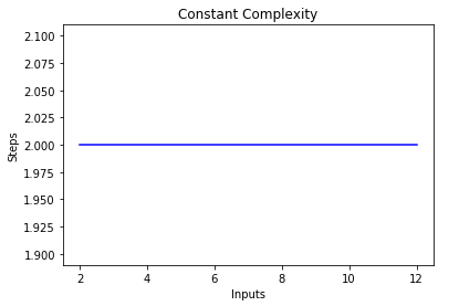
The complexity of an algorithm is said to be constant if the steps required to complete the execution of an algorithm remain constant, irrespective of the number of inputs. The constant complexity is denoted by O(c) where c can be any constant number.
Let's write a simple algorithm in Python that finds the square of the first item in the list and then prints it on the screen.
def constant_algo(items):
    result = items[0] * items[0]
    print ()

constant_algo([4, 5, 6, 8])
In the above script, irrespective of the input size, or the number of items in the input list items, the algorithm performs only 2 steps: Finding the square of the first element and printing the result on the screen. Hence, the complexity remains constant.
If you draw a line plot with the varying size of the items input on the x-axis and the number of steps on the y-axis, you will get a straight line. To visualize this, execute the following script:
import matplotlib.pyplot as plt
import numpy as np

x = [2, 4, 6, 8, 10, 12]

y = [2, 2, 2, 2, 2, 2]

plt.plot(x, y, 'b')
plt.xlabel('Inputs')
plt.ylabel('Steps')
plt.title('Constant Complexity')
plt.show()
Output:
Linear Complexity (O(n))
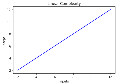
The complexity of an algorithm is said to be linear if the steps required to complete the execution of an algorithm increase or decrease linearly with the number of inputs. Linear complexity is denoted by O(n).
In this example, let's write a simple program that displays all items in the list to the console:
def linear_algo(items):
    for item in items:
        print(item)

linear_algo([4, 5, 6, 8])
The complexity of the linear_algo function is linear in the above example since the number of iterations of the for-loop will be equal to the size of the input items array. For instance, if there are 4 items in the items list, the for-loop will be executed 4 times, and so on.
The plot for linear complexity with inputs on x-axis and # of steps on the x-axis is as follows:
import matplotlib.pyplot as plt
import numpy as np

x = [2, 4, 6, 8, 10, 12]

y = [2, 4, 6, 8, 10, 12]

plt.plot(x, y, 'b')
plt.xlabel('Inputs')
plt.ylabel('Steps')
plt.title('Linear Complexity')
plt.show()
Output:
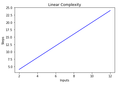
Another point to note here is that in case of a huge number of inputs the constants become insignificant. For instance, take a look at the following script:
def linear_algo(items):
    for item in items:
        print(item)

    for item in items:
        print(item)

linear_algo([4, 5, 6, 8])
In the script above, there are two for-loops that iterate over the input items list. Therefore the complexity of the algorithm becomes O(2n), however in case of infinite items in the input list, the twice of infinity is still equal to infinity, therefore we can ignore the constant 2 (since it is ultimately insignificant) and the complexity of the algorithm remains O(n).
We can further verify and visualize this by plotting the inputs on x-axis and the number of steps on y-axis as shown below:
import matplotlib.pyplot as plt
import numpy as np

x = [2, 4, 6, 8, 10, 12]

y = [4, 8, 12, 16, 20, 24]

plt.plot(x, y, 'b')
plt.xlabel('Inputs')
plt.ylabel('Steps')
plt.title('Linear Complexity')
plt.show()
In the script above, you can clearly see that y=2n, however the output is linear and looks like this:
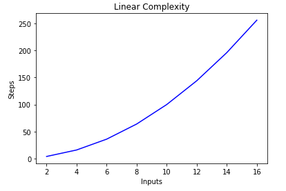
Quadratic Complexity (O(n^2))
The complexity of an algorithm is said to be quadratic when the steps required to execute an algorithm are a quadratic function of the number of items in the input. Quadratic complexity is denoted as O(n^2). Take a look at the following example to see a function with quadratic complexity:
def quadratic_algo(items):
    for item in items:
        for item2 in items:
            print(item, ' ' ,item)

quadratic_algo([4, 5, 6, 8])
In the script above, you can see that we have an outer loop that iterates through all the items in the input list and then a nested inner loop, which again iterates through all the items in the input list. The total number of steps performed is n * n, where n is the number of items in the input array.
The following graph plots the number of inputs vs the steps for an algorithm with quadratic complexity.
Finding the Complexity of Complex Functions
In the previous examples, we saw that only one function was being performed on the input. What if multiple functions are being performed on the input? Take a look at the following example.
def complex_algo(items):

    for i in range(5):
        print ("Python is awesome")

    for item in items:
        print(item)

    for item in items:
        print(item)

    print("Big O")
    print("Big O")
    print("Big O")

complex_algo([4, 5, 6, 8])
In the script above several tasks are being performed, first, a string is printed 5 times on the console using the print statement. Next, we print the input list twice on the screen and finally, another string is being printed three times on the console. To find the complexity of such an algorithm, we need to break down the algorithm code into parts and try to find the complexity of the individual pieces.
Let's break our script down into individual parts. In the first part we have:
    for i in range(5):
        print ("Python is awesome")
The complexity of this part is O(5). Since five constant steps are being performed in this piece of code irrespective of the input.
Next, we have:
    for item in items:
        print(item)
We know the complexity of above piece of code is O(n).
Similarly, the complexity of the following piece of code is also O(n)
    for item in items:
        print(item)
Finally, in the following piece of code, a string is being printed three times, hence the complexity is O(3)
    print("Big O")
    print("Big O")
    print("Big O")
To find the overall complexity, we simply have to add these individual complexities. Let's do so:
O(5) + O(n) + O(n) + O(3)
Simplifying above we get:
O(8) + O(2n)
We said earlier that when the input (which has length n in this case) becomes extremely large, the constants become insignificant i.e. twice or half of the infinity still remains infinity. Therefore, we can ignore the constants. The final complexity of the algorithm will be O(n).
Worst vs Best Case Complexity
Usually, when someone asks you about the complexity of the algorithm he is asking you about the worst case complexity. To understand the best case and worse case complexity, look at the following script:
def search_algo(num, items):
    for item in items:
        if item == num:
            return True
        else:
            return False
nums = [2, 4, 6, 8, 10]

print(search_algo(2, nums))
In the script above, we have a function that takes a number and a list of numbers as input. It returns true if the passed number is found in the list of numbers, otherwise it returns false. If you search 2 in the list, it will be found in the first comparison. This is the best case complexity of the algorithm that the searched item is found in the first searched index. The best case complexity, in this case, is O(1). On the other hand, if you search 10, it will be found at the last searched index. The algorithm will have to search through all the items in the list, hence the worst case complexity becomes O(n).
In addition to best and worst case complexity, you can also calculate the average complexity of an algorithm, which tells you "given a random input, what is the expected time complexity of the algorithm"?
Space Complexity
In addition to the time complexity, where you count the number of steps required to complete the execution of an algorithm, you can also find space complexity which refers to the number of spaces you need to allocate in the memory space during the execution of a program.
Have a look at the following example:
def return_squares(n):
    square_list = []
    return_squares
    for num in n:
        square_list.append(num * num)

    return square_list

nums = [2, 4, 6, 8, 10]
print(return_squares(nums))
In the script above, the function accepts a list of integers and returns a list with the corresponding squares of integers. The algorithm has to allocate memory for the same number of items as in the input list. Therefore, the space complexity of the algorithm becomes O(n).
Conclusion
The Big-O notation is the standard metric used to measure the complexity of an algorithm. In this article, we studied what Big-O notation is and how it can be used to measure the complexity of a variety of algorithms. We also studied different types of Big-O functions with the help of different Python examples. Finally, we briefly reviewed the worst and best case complexity along with the space complexity.
from Planet Python
via read more


No comments:
Post a Comment