Thursday, April 2, 2020

Red Hat Developers: How to write an ABI compliance checker using Libabigail

I’ve previously written about the challenges of ensuring forward compatibility for application binary interfaces (ABIs) exposed by native shared libraries. This article introduces the other side of the equation: How to verify ABI backward compatibility for upstream projects.

If you’ve read my previous article, you’ve already been introduced to Libabigail, a static-code analysis and instrumentation library for constructing, manipulating, serializing, and de-serializing ABI-relevant artifacts.

In this article, I’ll show you how to build a Python-based checker that uses Libabigail to verify the backward compatibility of ABIs in a shared library. For this case, we’ll focus on ABIs for shared libraries in the executable and linkable format (ELF) binary format that runs on Linux-based operating systems.

Note: This tutorial assumes that you have Libabigail and its associated command-line tools, abidw and abidiff installed and set up in your development environment. See the Libabigail documentation for a guide to getting and installing Libabigail.

Ensuring backward compatibility

If we state that the ABI of a newer version of a shared library is backward compatible, we’re assuring our users that ABI changes in the newer version of the library won’t affect applications linked against older versions. This means application functionality won’t change or be disrupted in any way, even for users who update to the newer version of the library without recompiling their application.

To make such a statement with confidence, we need a way to compare the ABI of the newer library version against the older one. Knowing what the ABI changes are, we’ll then be able to determine whether any change is likely to break backward compatibility.

The example project: libslicksoft.so

For the sake of this article, let’s assume I’m the release manager for a free software project named SlickSoftware. I have convinced you (my fellow hacker) that the ABI of our library, libslicksoft.so, should be backward compatible with older versions, at least for now.  In order to ensure backward compatibility, we’ll write an ABI-checking program that we can run at any point in the development cycle. The checker will help us ensure that the ABI for the current version of libslicksoft.so remains compatible with the ABI of a previous version, the baseline ABI. Once we’ve written the checker, we’ll also be able to use it for future projects.

Here’s the layout of the slick-software/lib directory, which contains SlickSoftware’s source code:

+ slick-software/
|
+ lib/
|    |
|    + file1.c
|    |
|    + Makefile
|
+ include/
|        |
|        + public-header.h
|
+ abi-ref/

Let’s start by setting up our example project.

Step 1: Create a shared library

To create a shared library, we visit the slick-software/lib directory and type make. We’ll call the new shared library slick-software/lib/libslicksoft.so.

Step 2: Create a representation of the reference ABI

Our next step is to create a representation of the ABI for our shared library, slick-software/lib/libslicksoft.so. Once we’ve done that, we’ll save it in the slick-software/abi-ref/ directory, which is currently empty.

The ABI representation will serve as a reference ABI. We’ll compare the ABI of all subsequent versions of libslicksoft.so against it. In theory, we could just save a copy of libslicksoft.so and use the binary itself for ABI comparisons.  We’ve chosen not to do that because, like many developers, we don’t like storing binaries in revision-control software. Luckily Libabigail allows us to save a textual representation of the ABI.

Creating the ABI representation

To generate a textual representation of an ELF binary’s ABI, all we have to do is open Libabigail’s command-line tool, abidw, and enter the following:

$ abidw slick-software/lib/libslicksoft.so > slick-software/abi-ref/libslicksoft.so.abi

Automating the creation process

We can automate this process by adding a rule at the end of slick-software/lib/Makefile. In the future, we’ll just type make abi-ref whenever we want to generate a textual representation of the ABI libslicksoft.so.abi file.

Here’s the content of that Makefile:

$cat slick-software/lib/Makefile SRCS:=file1.c
HEADER_FILE:=../include/public-header.h
SHARED_LIB:=libslicksoft.so
SHARED_LIB_SONAME=libslicksoft
ABI_REF_DIR=../abi-ref
ABI_REF=$(ABI_REF_DIR)/$(SHARED_LIB).abi
CFLAGS:=-Wall -g -I../include
LDFLAGS:=-shared -Wl,-soname=$(SHARED_LIB_SONAME)
ABIDW:= /usr/bin/abidw
ABIDIFF= /usr/bin/abidiff

OBJS:=$(subst .c,.o,$(SRCS))

all: $(SHARED_LIB)

%.o:%.c $(HEADER_FILE)
        $(CC) -c $(CFLAGS) -o $@ $<

$(SHARED_LIB): $(OBJS)
        $(CC) $(LDFLAGS) -o $@ $<

clean:
        rm -f *.o $(SHARED_LIB) $(ABI_REF)

abi-ref: $(SHARED_LIB)
        $(ABIDW) $< > $(ABI_REF)

Step 3: Compare ABI changes

Now that we have a reference ABI, we just need to compare newer versions of libslicksoft.so against it and analyze the changes. We can use Libabigail’s abidiff program to compare the two library versions. Here’s the command to invoke abidiff:

abidiff baseline.abi path/to/new-binary

This command line compares the ABIs of new-binary against the baseline.abi. It produces a report about the potential ABI changes, then returns a status code that tells us about the different kinds of ABI changes detected. By analyzing the status code, which is represented as a bitmap, we’ll be able to tell if any of the ABI changes are likely to break backward compatibility.

The Python-based ABI diff checker

Our next task is to write a program that invokes abidiff to perform the ABI check. We’ll call it check-abi and place it in the new slick-software/tools directory.

I’ve been told Python is cool, so I want to try it out with this new checker. I am far from being a Python expert, but hey, what can go wrong?

Step 1: Spec the ABI checker

To start, let’s walk through this Python-based ABI checker we want to write. We’ll run it like this:

$ check-abi baseline.abi slicksoft.so

The checker should be simple. If there are no ABI issues it will exit with a zero (0) status code. If it finds a backward-compatibility issue, it will return a non-zero status code and a useful message.

Step 2: Import dependencies

We’re writing the check-abi program as a script in Python 3. The first thing we’ll do is import the packages we need for this program:

#!/usr/bin/env python3

import argparse
import subprocess
import sys

Step 3: Define a parser

Next, we’ll need a function that parses command-line arguments. Let’s define it without bothering too much about the content for now:

def parse_command_line():
    """Parse the command line arguments.

       check-abi expects the path to the new binary and a path to the
       baseline ABI to compare against.  It can also optionaly take
       the path to the abidiff program to use.
    """
# ...

Step 4: Write the main function

In this case, I’ve already written the main function, so let’s take a look:

def main():
    # Get the configuration of this program from the command line
    # arguments. The configuration ends up being a variable named
    # config, which has three properties:
    #
    #   config.abidiff: this is the path to the abidiff program
    #
    #   config.baseline_abi: this is the path to the baseline
    #                        ABI. It's the reference ABI that was
    #                        previously stored and that we need to
    #                        compare the ABI of the new binary
    #                        against.
    #
    #   config.new_abi: this is the path to the new binary which ABI
    #                   is to be compared against the baseline
    #                   referred to by config.baseline_abi.
    #
    config = parse_command_line()

    # Execute the abidiff program to compare the new ABI against the
    # baseline.
    completed_process = subprocess.run([config.abidiff,
                                        "--no-added-syms",
                                        config.baseline_abi,
                                        config.new_abi],
                                       universal_newlines = True,
                                       stdout = subprocess.PIPE,
                                       stderr = subprocess.STDOUT)

    if completed_process.returncode != 0:
        # Let's define the values of the bits of the "return code"
        # returned by abidiff.  Depending on which bit is set, we know
        # what happened in terms of ABI verification.  These bits are
        # documented at
        # https://sourceware.org/libabigail/manual/abidiff.html#return-values.
        ABIDIFF_ERROR_BIT = 1
        ABI_CHANGE_BIT = 4
        ABI_INCOMPATIBLE_CHANGE_BIT = 8

        if completed_process.returncode & ABIDIFF_ERROR_BIT:
            print("An unexpected error happened while running abidiff:\n")
            return 0
        elif completed_process.returncode & ABI_INCOMPATIBLE_CHANGE_BIT:
            # If this bit is set, it means we detected an ABI change
            # that breaks backwards ABI compatibility, for sure.
            print("An incompatible ABI change was detected:\n")
        elif completed_process.returncode & ABI_CHANGE_BIT:
            # If this bit is set, (and ABI_INCOMPATIBLE_CHANGE_BIT is
            # not set) then it means there was an ABI change that
            # COULD potentially break ABI backward compatibility.  To
            # be sure if this change is problematic or not, a human
            # review is necessary
            print("An ABI change that needs human review was detected:\n")

        print("%s" % completed_process.stdout)
        return completed_process.returncode

    return 0;

Notes about the code

The code is heavily commented to make it easier for future programmers to understand. Here are two important highlights. First, notice how check-abi invokes abidiff with the --no-added-syms option. That option tells abidiff that added functions, global variables, and publicly defined ELF symbols (aka added ABI artifacts) should not be reported. This lets us focus our attention on ABI artifacts that have been changed or removed.

Second, notice how we’ve set the checker to analyze the return code generated by abidiff. You can see this detail in the if statement starting here:

if completed_process.returncode != 0:

If the first bit of that return code is set (bit value 1) then it means abidiff encountered a plumbing error while executing. In that case, check-abi will print an error message but it won’t report an ABI issue.

If the fourth bit of the return code is set (bit value 8) then it means an ABI change breaks backward compatibility with the older library version. In that case, check-abi will print a meaningful message and a detailed report of the change. Recall that in this case, the checker produces a non-zero return code.

If only the third bit of the return code is set (bit value 4), and the fourth bit mentioned above is not, then it means abidiff detected an ABI change that could potentially break backward compatibility. In this case, a human review of the change is necessary. The checker will print a meaningful message and a detailed report for someone to review.

Note: If you are interested, you can find the complete details of the return code generated by abidiff here.

Source code for the check-abi program

Here’s the complete source code for the check-abi program:

#!/usr/bin/env python3

import argparse
import subprocess
import sys

def parse_command_line():
    """Parse the command line arguments.

       check-abi expects the path to the new binary and a path to the
       baseline ABI to compare against.  It can also optionaly take
       the path to the abidiff program to use.
    """

    parser = argparse.ArgumentParser(description="Compare the ABI of a binary "
                                                 "against a baseline")
    parser.add_argument("baseline_abi",
                        help = "the path to a baseline ABI to compare against")
    parser.add_argument("new_abi",
                        help = "the path to the ABI to compare "
                               "against the baseline")
    parser.add_argument("-a",
                        "--abidiff",
                        required = False,
                        default="/home/dodji/git/libabigail/master/build/tools/abidiff")

    return parser.parse_args()


def main():
    # Get the configuration of this program from the command line
    # arguments. The configuration ends up being a variable named
    # config, which has three properties:
    #
    #   config.abidiff: this is the path to the abidiff program
    #
    #   config.baseline_abi: this is the path to the baseline
    #                        ABI. It's the reference ABI that was
    #                        previously stored and that we need to
    #                        compare the ABI of the new binary
    #                        against.
    #
    #   config.new_abi: this is the path to the new binary which ABI
    #                   is to be compared against the baseline
    #                   referred to by config.baseline_abi.
    #
    config = parse_command_line()

    # Execute the abidiff program to compare the new ABI against the
    # baseline.
    completed_process = subprocess.run([config.abidiff,
                                        "--no-added-syms",
                                        config.baseline_abi,
                                        config.new_abi],
                                       universal_newlines = True,
                                       stdout = subprocess.PIPE,
                                       stderr = subprocess.STDOUT)

    if completed_process.returncode != 0:
        # Let's define the values of the bits of the "return code"
        # returned by abidiff.  Depending on which bit is set, we know
        # what happened in terms of ABI verification.  These bits are
        # documented at
        # https://sourceware.org/libabigail/manual/abidiff.html#return-values.
        ABIDIFF_ERROR_BIT = 1
        ABI_CHANGE_BIT = 4
        ABI_INCOMPATIBLE_CHANGE_BIT = 8

        if completed_process.returncode & ABIDIFF_ERROR_BIT:
            print("An unexpected error happened while running abidiff:\n")
            return 0
        elif completed_process.returncode & ABI_INCOMPATIBLE_CHANGE_BIT:
            # If this bit is set, it means we detected an ABI change
            # that breaks backwards ABI compatibility, for sure.
            print("An incompatible ABI change was detected:\n")
        elif completed_process.returncode & ABI_CHANGE_BIT:
            # If this bit is set, (and ABI_INCOMPATIBLE_CHANGE_BIT is
            # not set) then it means there was an ABI change that
            # COULD potentially break ABI backward compatibility.  To
            # be sure if this change is problematic or not, a human
            # review is necessary
            print("An ABI change that needs human review was detected:\n")

        print("%s" % completed_process.stdout)
        return completed_process.returncode

    return 0;

if __name__ == "__main__":
    sys.exit(main())

Using check-abi from the Makefile

We’re done with our basic checker, but we could add a feature or two. For instance, wouldn’t it be nice if we could invoke our shiny new check-abi program from the slick-software/lib directory? Then we could enter a simple make command anytime we needed to do an ABI verification.

We can set this feature up by adding a rule at the end of the slick-software/lib/Makefile:

abi-check: $(SHARED_LIB)
        $(CHECK_ABI) $(ABI_REF) $(SHARED_LIB) || echo "ABI compatibility issue detected!"

Of course, we also need to define the variable CHECK_ABI at the beginning of the Makefile:

CHECK_ABI=../tools/check-abi

Here’s the complete Makefile with these changes:

SRCS:=file1.c
HEADER_FILE:=../include/public-header.h
SHARED_LIB:=libslicksoft.so
SHARED_LIB_SONAME=libslicksoft
ABI_REF_DIR=../abi-ref
ABI_REF=$(ABI_REF_DIR)/$(SHARED_LIB).abi
CFLAGS:=-Wall -g -I../include
LDFLAGS:=-shared -Wl,-soname=$(SHARED_LIB_SONAME)
ABIDW:=/usr/bin/abidw
ABIDIFF=/usr/bin/abidiff
CHECK_ABI=../tools/check-abi

OBJS:=$(subst .c,.o,$(SRCS))

all: $(SHARED_LIB)

%.o:%.c $(HEADER_FILE)
        $(CC) -c $(CFLAGS) -o $@ $<

$(SHARED_LIB): $(OBJS)
        $(CC) $(LDFLAGS) -o $@ $<

clean:
        rm -f *.o $(SHARED_LIB) $(ABI_REF)

abi-ref: $(SHARED_LIB)
        $(ABIDW) $< > $(ABI_REF)

abi-check: $(SHARED_LIB)
        $(CHECK_ABI) $(ABI_REF) $(SHARED_LIB) || echo "ABI compatibility issue detected!"

Run the checker

We’re nearly done, but let’s test our new checker with a simple ABI check for backward compatibility. First, I will make a few changes to the slick-software library, so I have differences to check.

Next, I visit the slick-software/lib directory and run make abi-check. Here’s what’s I get back:

$ make abi-check
../tools/check-abi ../abi-ref/libslicksoft.so.abi libslicksoft.so || echo "ABI compatibility issue detected!"
An incompatible ABI change was detected:

Functions changes summary: 1 Removed, 0 Changed, 0 Added function
Variables changes summary: 0 Removed, 0 Changed, 0 Added variable

1 Removed function:

  'function void function_1()'    {function_1}

ABI compatibility issue detected!
$

The ABI checker is reporting one compatibility issue, with a removed function. I guess I should put function_1() back in to avoid breaking the ABI.

Conclusion

In this article, I showed you how to write a basic ABI verifier for shared libraries in your upstream projects. To keep this project simple, I left out other features that you might want to add to the checker yourself. For instance, Libabigail has mechanisms for handling false positives, which are common in real-world projects. Also, we are constantly improving this tool for the quality of the analysis it can do. If anything about Libabigail doesn’t work as you would like, please let us know on the Libabigail mailing list.

Happy hacking, and may all of your ABI incompatibilities be spotted.

Share

The post How to write an ABI compliance checker using Libabigail appeared first on Red Hat Developer.


from Planet Python
via read more

Wednesday, April 1, 2020

Python Folder Sync

Python Folder Sync. Sync-It is a friendly Windows only systray app to sync two folders as and when required.

from Python Coder
via read more

Stack Abuse: One-Hot Encoding in Python with Pandas and Scikit-Learn

Introduction

In computer science, data can be represented in a lot of different ways, and naturally, every single one of them has its advantages as well as disadvantages in certain fields.

Since computers are unable to process categorical data as these categories have no meaning for them, this information has to be prepared if we want a computer to be able to process it.

This action is called preprocessing. A big part of preprocessing is encoding - representing every single piece of data in a way that a computer can understand (the name literally means "convert to computer code").

In many branches of computer science, especially machine learning and digital circuit design, One-Hot Encoding is widely used.

In this article, we will explain what one-hot encoding is and implement it in Python using a few popular choices, Pandas and Scikit-Learn. We'll also compare it's effectiveness to other types of representation in computers, its strong points and weaknesses, as well as its applications.

What is One-Hot Encoding?

One-hot Encoding is a type of vector representation in which all of the elements in a vector are 0, except for one, which has 1 as its value, where 1 represents a boolean specifying a category of the element.

There also exists a similar implementation called One-Cold Encoding, where all of the elements in a vector are 1, except for one, which has 0 as its value.

For instance, [0, 0, 0, 1, 0] and [1 ,0, 0, 0, 0] could be some examples of one-hot vectors. A similar technique to this one, also used to represent data, would be dummy variables in statistics.

This is very different from other encoding schemes, which all allow multiple bits to have 1 as its value. Below is a table that compares the representation of numbers from 0 to 7 in binary, Gray code, and one-hot:

Decimal Binary Gray code One-Hot
0 000 000 0000000
1 001 001 0000001
2 010 011 0000010
3 011 010 0000100
4 100 110 0001000
5 101 111 0010000
6 110 101 0100000
7 111 100 1000000

Practically, for every one-hot vector, we ask n questions, where n is the number of categories we have:

Is this the number 1? Is this the number 2? ... Is this the number 7?

Each "0" is "false" and once we hit a "1" in a vector, the answer to the question is "true".

One-hot encoding transforms categorical features to a format that works better with classification and regression algorithms. It's very useful in methods where multiple types of data representation is necessary.

For example, some vectors may be optimal for regression (approximating functions based on former return values), and some may be optimal for classification (categorization into fixed sets/classes, typically binary):

Label ID
Strawberry 1
Apple 2
Watermelon 3
Lemon 4
Peach 5
Orange 6

Here we have six sample inputs of categorical data. The type of encoding used here is called "label encoding" - and it is very simple: we just assign an ID for a categorical value.

Our computer now knows how to represent these categories, because it knows how to work with numbers. However, this method of encoding is not very effective, because it tends to naturally give the higher numbers higher weights.

It wouldn't make sense to say that our category of "Strawberries" is greater or smaller than "Apples", or that adding the category "Lemon" to "Peach" would give us a category "Orange", since these values are not ordinal.

If we represented these categories in one-hot encoding, we would actually replace the rows with columns. We do this by creating one boolean column for each of our given categories, where only one of these columns could take on the value 1 for each sample:

Strawberry Apple Watermelon Lemon Peach Orange ID
1 0 0 0 0 0 1
0 1 0 0 0 0 2
0 0 1 0 0 0 3
0 0 0 1 0 0 4
0 0 0 0 1 0 5
0 0 0 0 0 1 6

We can see from the tables above that more digits are needed in one-hot representation compared to Binary or Gray code. For n digits, one-hot encoding can only represent n values, while Binary or Gray encoding can represent 2n values using n digits.

Implementation

Pandas

Let's take a look at a simple example of how we can convert values from a categorical column in our dataset into their numerical counterparts, via the one-hot encoding scheme.

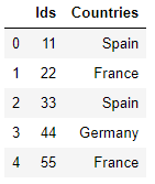
We'll be creating a really simple dataset - a list of countries and their ID's:

import pandas as pd

ids = [11, 22, 33, 44, 55, 66, 77]
countries = ['Spain', 'France', 'Spain', 'Germany', 'France']

df = pd.DataFrame(list(zip(ids, countries)),
                  columns=['Ids', 'Countries'])

In the script above, we create a Pandas dataframe, called df using two lists i.e. ids and countries. If you call the head() method on the dataframe, you should see the following result:

df.head()

dataframe header one hot encoding

The Countries column contain categorical values. We can convert the values in the Countries column into one-hot encoded vectors using the get_dummies() function:

y = pd.get_dummies(df.Countries, prefix='Country')
print(y.head())

We passed Country as the value for the prefix attribute of the get_dummies() method, hence you can see the string Country prefixed before the header of each of the one-hot encoded columns in the output.

Running this code yields:

   Country_France  Country_Germany  Country_Spain
0               0                0              1
1               1                0              0
2               0                0              1
3               0                1              0
4               1                0              0

Scikit-Learn

An alternative would be to use another popular library - Scikit-Learn. It offers both the OneHotEncoder class and the LabelBinarizer class for this purpose.

First, let's start by importing the LabelBinarizer:

from sklearn.preprocessing import LabelBinarizer

And then, using the same dataframe as before, let's instantiate the LabelBinarizer and fit it:

y = LabelBinarizer().fit_transform(df.Countries)

Printing y would yield:

[[0 0 1]
 [1 0 0]
 [0 0 1]
 [0 1 0]
 [1 0 0]]

Though, this isn't nearly as pretty as the Pandas approach.

Similarly, we can use the OneHotEncoder class, which supports multi-column data, unlike the previous class:

from sklearn.preprocessing import OneHotEncoder

And then, let's populate a list and fit it in the encoder:

x = [[11, "Spain"], [22, "France"], [33, "Spain"], [44, "Germany"], [55, "France"]]
y = OneHotEncoder().fit_transform(x).toarray()
print(y)

Running this will yield:

[[1. 0. 0. 0. 0. 0. 0. 1.]
 [0. 1. 0. 0. 0. 1. 0. 0.]
 [0. 0. 1. 0. 0. 0. 0. 1.]
 [0. 0. 0. 1. 0. 0. 1. 0.]
 [0. 0. 0. 0. 1. 1. 0. 0.]]

Applications of One-Hot Encoding

One-hot encoding has seen most of its application in the fields of Machine Learning and Digital Circuit Design.

Machine Learning

As stated above, computers aren't very good with categorical data. While we understand categorical data just fine, it's due to a kind of prerequisite knowledge that computers don't have.

Most Machine Learning techniques and models work with a very bounded dataset (typically binary). Neural networks consume data and produce results in the range of 0..1 and rarely will we ever go beyond that scope.

In short, the vast majority of machine learning algorithms receive sample data ("training data") from which features are extracted. Based on these features, a mathematical model is created, which is then used to make predictions or decisions without being explicitly programmed to perform these tasks.

A great example would be Classification, where the input can be technically unbounded, but the output is typically limited to a few classes. In the case of binary classification (say we're teaching a neural network to classify cats and dogs), we'd have a mapping of 0 for cats, and 1 for dogs.

Most of the time, the training data we wish to perform predictions on is categorical, like the example with fruit mentioned above. Again, while this makes a lot of sense to us, the words themselves are of no meaning to the algorithm as it doesn't understand them.

Using one-hot encoding for representation of data in these algorithms is not technically necessary, but pretty useful if we want an efficient implementation.

Digital Circuit Design

Many basic digital circuits use one-hot notation in order to represent their I/O values.

For example, it can be used to indicate the state of a finite-state machine. If some other type of representation, like Gray or Binary, is used, a decoder is needed to determine the state as they're not as naturally compatible. Contrarily, a one-hot finite-state machine does not need the decoder, because if the nth bit is high, the machine is, logically, in the nth state.

A good example of a finite-state machine is a ring counter - a type of counter composed of flip-flops connected to a shift register, in which the output of one flip-flop connects to the input of the other one.

The first flip-flop in this counter represents the first state, the second represents the second state, and so on. At the beginning, all of the flip-flops in the machine are set to '0', except for the first one, which is set to '1'.

The next clock edge arriving at the flip flops advances the one 'hot' bit to the second flip flop. The 'hot' bit advances like this until the last state, after which the machine returns to the first state.

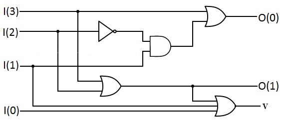
Another example of usage of one-hot encoding in digital circuit design would be an address decoder, which takes a Binary or Gray code input, and then converts it to one-hot for the output, as well as a priority encoder (shown in the picture below).

It's the exact opposite and takes the one-hot input and converts it to Binary or Gray:

digital circuit design

Advantages and Disadvantages of One-hot encoding

Like every other type of encoding, one-hot has many good points as well as problematic aspects.

Advantages

A great advantage of one-hot encoding is that determining the state of a machine has a low and constant cost, because all it needs to do is access one flip-flop. Changing the state of the machine is almost as fast, since it just needs to access two flip-flops.

Another great thing about one-hot encoding is the easy implementation. Digital circuits made in this notation are very easy to design and modify. Illegal states in the finite-state machine are also easy to detect.

A one-hot implementation is known for being the fastest one, allowing a state machine to run at a faster clock rate than any other encoding of that state machine.

Disadvantages

One of the main disadvantages that one-hot encoding has is the above mentioned fact that it can't represent many values (for n states, we would need n digits - or flip-flops). This is why, if we wanted to implement a one-hot 15-state ring counter for example, we would need 15 flip-flops, whereas the binary implementation would only need three flip-flops.

This makes it especially impractical for PAL devices, and it can also be very expensive, but it takes advantage of an FPGA's abundant flip-flops.

Another problem with this type of encoding is that many of the states in a finite-state machine would illegal - for every n valid states, there is (2n - n) illegal ones. A good thing is that these illegal states are, as previously said, really easy to detect (one XOR gate would be enough), so it's not very hard to take care of them.

Conclusion

Since one-hot encoding is very simple, it is easy to understand and use in practice. It's no surprise that it is this popular in the world of computer science.

Due to the fact that the cons aren't too bad, its seen wide application. At the end of the day, its pros clearly outweigh the cons, which is why this type of implementation will definitely stick around for a long time in the future.


from Planet Python
via read more

Python Software Foundation: An Update on PyPI Funded Work

Originally announced at the end of 2018, a gift from Facebook Research is funding improvements for the security PyPI and its users.

What's been done

After launching a request for information and subsequent request for proposal in the second half of 2019, contractors were selected and work commenced on Milestone 2 of the project in December 2019 and was completed in February 2020.
The result is that PyPI now has tooling in place to implement automated checks that run in response to events such as Project or Release creation or File uploads as well as on schedules. In addition to documentation example checks were also implemented that demonstrate event based and scheduled checks.
Results from checks are made available for PyPI moderators and administrators to review, but will not have any automated responses put in place. As a check suite is developed and refined we hope that these will help to identify malicious uploads and spam that PyPI regularly contends with.

What's next

With the acceptance of PEP 458 on February 15 we're excited to announce that work on implementation of The Update Framework has started.
This work will enable clients like pip to ensure that they have downloaded valid files from PyPI and equip the PyPI administrators to better respond in event of a compromise.
The timeline for this work is currently planned over the coming months, with an initial key signing to be held at PyCon 2020 in Pittsburgh, Pennsylvania and rollout of the services needed to support TUF enabled clients in May or June.

Other PyPI News

For users who have enabled two factor authentication on PyPI, support has been added for Account Recovery codes. These codes are intended for use in the case where you've lost your Webauthn device or TOTP application, allowing you to recover access to your account.
You can generate and store recovery codes now by visiting your account settings and clicking "Generate Recovery Codes".


from Planet Python
via read more

Real Python: Linked Lists in Python: An Introduction

Linked lists are like a lesser-known cousin of lists. They’re not as popular or as cool, and you might not even remember them from your algorithms class. But in the right context, they can really shine.

In this article, you’ll learn:

  • What linked lists are and when you should use them
  • How to use collections.deque for all of your linked list needs
  • How to implement your own linked lists
  • What the other types of linked lists are and what they can be used for

If you’re looking to brush up on your coding skills for a job interview, or if you want to learn more about Python data structures besides the usual dictionaries and lists, then you’ve come to the right place!

You can follow along with the examples in this tutorial by downloading the source code available at the link below:

Get the Source Code: Click here to get the source code you'll use to learn about linked lists in this tutorial.

Understanding Linked Lists

Linked lists are an ordered collection of objects. So what makes them different from normal lists? Linked lists differ from lists in the way that they store elements in memory. While lists use a contiguous memory block to store references to their data, linked lists store references as part of their own elements.

Main Concepts

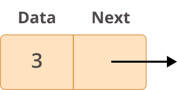
Before going more in depth on what linked lists are and how you can use them, you should first learn how they are structured. Each element of a linked list is called a node, and every node has two different fields:

  1. Data contains the value to be stored in the node.
  2. Next contains a reference to the next node on the list.

Here’s what a typical node looks like:

Example Node of a Linked ListNode

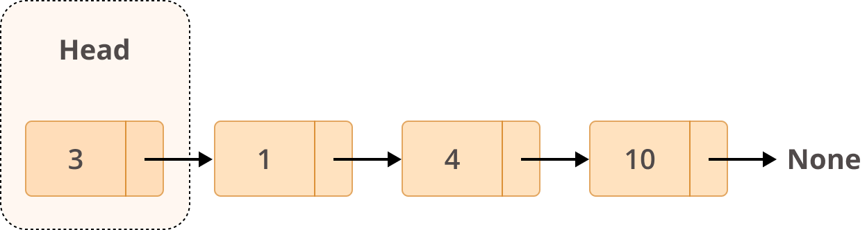
A linked list is a collection of nodes. The first node is called the head, and it’s used as the starting point for any iteration through the list. The last node must have its next reference pointing to None to determine the end of the list. Here’s how it looks:

Example Structure of a Linked ListLinked List

Now that you know how a linked list is structured, you’re ready to look at some practical use cases for it.

Practical Applications

Linked lists serve a variety of purposes in the real world. They can be used to implement (spoiler alert!) queues or stacks as well as graphs. They’re also useful for much more complex tasks, such as lifecycle management for an operating system application.

Queues or Stacks

Queues and stacks differ only in the way elements are retrieved. For a queue, you use a First-In/First-Out (FIFO) approach. That means that the first element inserted in the list is the first one to be retrieved:

Example Structure of a QueueQueue

In the diagram above, you can see the front and rear elements of the queue. When you append new elements to the queue, they’ll go to the rear end. When you retrieve elements, they’ll be taken from the front of the queue.

For a stack, you use a Last-In/Fist-Out (LIFO) approach, meaning that the last element inserted in the list is the first to be retrieved:

Example Structure of a StackStack

In the above diagram you can see that the first element inserted on the stack (index 0) is at the bottom, and the last element inserted is at the top. Since stacks use the LIFO approach, the last element inserted (at the top) will be the first to be retrieved.

Because of the way you insert and retrieve elements from the edges of queues and stacks, linked lists are one of the most convenient ways to implement these data structures. You’ll see examples of these implementations later in the article.

Graphs

Graphs can be used to show relationships between objects or to represent different types of networks. For example, a visual representation of a graph—say a directed acyclic graph (DAG)—might look like this:

Example Directed GraphDirected Acyclic Graph

There are different ways to implement graphs like the above, but one of the most common is to use an adjacency list. An adjacency list is, in essence, a list of linked lists where each vertex of the graph is stored alongside a collection of connected vertices:

Vertex Linked List of Vertices
1 2 → 3 → None
2 4 → None
3 None
4 5 → 6 → None
5 6 → None
6 None

In the table above, each vertex of your graph is listed in the left column. The right column contains a series of linked lists storing the other vertices connected with the corresponding vertex in the left column. This adjacency list could also be represented in code using a dict:

>>>
>>> graph = {
...     1: [2, 3, None],
...     2: [4, None],
...     3: [None],
...     4: [5, 6, None],
...     5: [6, None],
...     6: [None]
... }

The keys of this dictionary are the source vertices, and the value for each key is a list. This list is usually implemented as a linked list.

Note: In the above example you could avoid storing the None values, but we’ve retained them here for clarity and consistency with later examples.

In terms of both speed and memory, implementing graphs using adjacency lists is very efficient in comparison with, for example, an adjacency matrix. That’s why linked lists are so useful for graph implementation.

Performance Comparison: Lists vs Linked Lists

In most programming languages, there are clear differences in the way linked lists and arrays are stored in memory. In Python, however, lists are dynamic arrays. That means that the memory usage of both lists and linked lists is very similar.

Further reading: Python’s implementation of dynamic arrays is quite interesting and definitely worth a read. Make sure to have a look and use that knowledge to stand out at your next company party!

Since the difference in memory usage between lists and linked lists is so insignificant, it’s better if you focus on their performance differences when it comes to time complexity.

Insertion and Deletion of Elements

List insertion times vary depending on the need to resize the existing array. If you read the article above on how lists are implemented, then you’ll notice that Python overallocates space for arrays based on their growth. This means that inserting a new element into a list can take anywhere from Θ(n) to Θ(1) depending on whether the existing array needs to be resized.

The same applies for deleting elements from the array. If the size of the array is less than half the allocated size, then Python will shrink the array. So, all in all, inserting or deleting elements from an array has an average time complexity of Θ(n).

Linked lists, however, are much better when it comes to insertion and deletion of elements at the beginning or the end of the list, where their time complexity is constant: Θ(1). This performance advantage is the reason linked lists are so useful for queues and stacks, where elements are continuously inserted and removed from the edges.

Retrieval of Elements

When it comes to element lookup, lists perform much better than linked lists. When you know which element you want to access, lists can perform this operation in Θ(1) time. Trying to do the same with a linked list would take Θ(n) because you need to traverse the whole list to find the element.

When searching for a specific element, however, both lists and linked lists perform very similarly, with a time complexity of Θ(n). In both cases, you need to iterate through the entire list to find the element you’re looking for.

Introducing collections.deque

In Python, there’s a specific object in the collections module that you can use for linked lists called deque(pronounced “deck”), which stands for double-ended queue.

collections.deque uses an implementation of a linked list in which you can access, insert, or remove elements from the beginning or end of a list with constant O(1) performance.

How to Use collections.deque

There are quite a few methods that come, by default, with a deque object. However, in this article you’ll only touch on a few of them, mostly for adding or removing elements.

First, you need to create a linked list. You can use the following piece of code to do that with deque:

>>>
>>> from collections import deque
>>> deque()
deque([])

The code above will create an empty linked list. If you want to populate it at creation, then you can give it an iterable as input:

>>>
>>> deque(['a','b','c'])
deque(['a', 'b', 'c'])

>>> deque('abc')
deque(['a', 'b', 'c'])

>>> deque([{'data': 'a'}, {'data': 'b'}])
deque([{'data': 'a'}, {'data': 'b'}])

When initializing a deque object, you can pass any iterable as an input, such as a string (also an iterable) or a list of objects.

Now that you know how to create a deque object, you can interact with it by adding or removing elements. You can create an abcde linked list and add a new element f like this:

>>>
>>> llist = deque("abcde")
>>> llist
deque(['a', 'b', 'c', 'd', 'e'])

>>> llist.append("f")
>>> llist
deque(['a', 'b', 'c', 'd', 'e', 'f'])

>>> llist.pop()
'f'

>>> llist
deque(['a', 'b', 'c', 'd', 'e'])

Both append() and pop() add or remove elements from the right side of the linked list. However, you can also use deque to quickly add or remove elements from the left side, or head, of the list:

>>>
>>> llist.appendleft("z")
>>> llist
deque(['z', 'a', 'b', 'c', 'd', 'e'])

>>> llist.popleft()
'z'

>>> llist
deque(['a', 'b', 'c', 'd', 'e'])

Adding or removing elements from both ends of the list is pretty straightforward using the deque object. Now you’re ready to learn how to use collections.deque to implement a queue or a stack.

How to Implement Queues and Stacks

As you learned above, the main difference between a queue and a stack is the way you retrieve elements from each. Next, you’ll find out how to use collections.deque to implement both data structures.

Queues

With queues, you want to add values to a list (enqueue), and when the timing is right, you want to remove the element that has been on the list the longest (dequeue). For example, imagine a queue at a trendy and fully booked restaurant. If you were trying to implement a fair system for seating guests, then you’d start by creating a queue and adding people as they arrive:

>>>
>>> from collections import deque
>>> queue = deque()
>>> queue
deque([])

>>> queue.append("Mary")
>>> queue.append("John")
>>> queue.append("Susan")
>>> queue
deque(['Mary', 'John', 'Susan'])

Now you have Mary, John, and Susan in the queue. Remember that since queues are FIFO, the first person who got into the queue should be the first to get out.

Now imagine some time goes by and a few tables become available. At this stage, you want to remove people from the queue in the correct order. This is how you would do that:

>>>
>>> queue.popleft()
'Mary'

>>> queue
deque(['John', 'Susan'])

>>> queue.popleft()
'John'

>>> queue
deque(['Susan'])

Every time you call popleft(), you remove the head element from the linked list, mimicking a real-life queue.

Stacks

What if you wanted to create a stack instead? Well, the idea is more or less the same as with the queue. The only difference is that the stack uses the LIFO approach, meaning that the last element to be inserted in the stack should be the first to be removed.

Imagine you’re creating a web browser’s history functionality in which store every page a user visits so they can go back in time easily. Assume these are the actions a random user takes on their browser:

  1. Visits Real Python’s website
  2. Navigates to Pandas: How to Read and Write Files
  3. Clicks on a link for Reading and Writing CSV Files in Python

If you’d like to map this behavior into a stack, then you could do something like this:

>>>
>>> from collections import deque
>>> history = deque()

>>> history.appendleft("https://realpython.com/")
>>> history.appendleft("https://realpython.com/pandas-read-write-files/")
>>> history.appendleft("https://realpython.com/python-csv/")
>>> history
deque(['https://realpython.com/python-csv/',
       'https://realpython.com/pandas-read-write-files/',
       'https://realpython.com/'])

In this example, you created an empty history object, and every time the user visited a new site, you added it to your history variable using appendleft(). Doing so ensured that each new element was added to the head of the linked list.

Now suppose that after the user read both articles, they wanted to go back to the Real Python home page to pick a new article to read. Knowing that you have a stack and want to remove elements using LIFO, you could do the following:

>>>
>>> history.popleft()
'https://realpython.com/python-csv/'

>>> history.popleft()
'https://realpython.com/pandas-read-write-files/'

>>> history
deque(['https://realpython.com/'])

There you go! Using popleft(), you removed elements from the head of the linked list until you reached the Real Python home page.

From the examples above, you can see how useful it can be to have collections.deque in your toolbox, so make sure to use it the next time you have a queue- or stack-based challenge to solve.

Implementing Your Own Linked List

Now that you know how to use collections.deque for handling linked lists, you might be wondering why you would ever implement your own linked list in Python. There are a few reasons to do it:

  1. Practicing your Python algorithm skills
  2. Learning about data structure theory
  3. Preparing for job interviews

Feel free to skip this next section if you’re not interested in any of the above, or if you already aced implementing your own linked list in Python. Otherwise, it’s time to implement some linked lists!

How to Create a Linked List

First things first, create a class to represent your linked list:

class LinkedList:
    def __init__(self):
        self.head = None

The only information you need to store for a linked list is where the list starts (the head of the list). Next, create another class to represent each node of the linked list:

class Node:
    def __init__(self, data):
        self.data = data
        self.next = None

In the above class definition, you can see the two main elements of every single node: data and next. You can also add a __repr__ to both classes to have a more helpful representation of the objects:

class Node:
    def __init__(self, data):
        self.data = data
        self.next = None

    def __repr__(self):
        return self.data

class LinkedList:
    def __init__(self):
        self.head = None

    def __repr__(self):
        node = self.head
        nodes = []
        while node is not None:
            nodes.append(node.data)
            node = node.next
        nodes.append("None")
        return " -> ".join(nodes)

Have a look at an example of using the above classes to quickly create a linked list with three nodes:

>>>
>>> llist = LinkedList()
>>> llist
None

>>> first_node = Node("a")
>>> llist.head = first_node
>>> llist
a -> None

>>> second_node = Node("b")
>>> third_node = Node("c")
>>> first_node.next = second_node
>>> second_node.next = third_node
>>> llist
a -> b -> c -> None

By defining a node’s data and next values, you can create a linked list quite quickly. These LinkedList and Node classes are the starting points for our implementation. From now on, it’s all about increasing their functionality.

Here’s a slight change to the linked list’s __init__() that allows you to quickly create linked lists with some data:

def __init__(self, nodes=None):
    self.head = None
    if nodes is not None:
        node = Node(data=nodes.pop(0))
        self.head = node
        for elem in nodes:
            node.next = Node(data=elem)
            node = node.next

With the above modification, creating linked lists to use in the examples below will be much faster.

How to Traverse a Linked List

One of the most common things you will do with a linked list is to traverse it. Traversing means going through every single node, starting with the head of the linked list and ending on the node that has a next value of None.

Traversing is just a fancier way to say iterating. So, with that in mind, create an __iter__ to add the same behavior to linked lists that you would expect from a normal list:

def __iter__(self):
    node = self.head
    while node is not None:
        yield node
        node = node.next

The method above goes through the list and yields every single node. The most important thing to remember about this __iter__ is that you need to always validate that the current node is not None. When that condition is True, it means you’ve reached the end of your linked list.

After yielding the current node, you want to move to the next node on the list. That’s why you add node = node.next. Here’s an example of traversing a random list and printing each node:

>>>
>>> llist = LinkedList(["a", "b", "c", "d", "e"])
>>> llist
a -> b -> c -> d -> e -> None

>>> for node in llist:
...     print(node)
a
b
c
d
e

In other articles, you might see the traversing defined into a specific method called traverse(). However, using Python’s built-in methods to achieve said behavior makes this linked list implementation a bit more Pythonic.

How to Insert a New Node

There are different ways to insert new nodes into a linked list, each with its own implementation and level of complexity. That’s why you’ll see them split into specific methods for inserting at the beginning, end, or between nodes of a list.

Inserting at the Beginning

Inserting a new node at the beginning of a list is probably the most straightforward insertion since you don’t have to traverse the whole list to do it. It’s all about creating a new node and then pointing the head of the list to it.

Have a look at the following implementation of add_first() for the class LinkedList:

def add_first(self, node):
    node.next = self.head
    self.head = node

In the above example, you’re setting self.head as the next reference of the new node so that the new node points to the old self.head. After that, you need to state that the new head of the list is the inserted node.

Here’s how it behaves with a sample list:

>>>
>>> llist = LinkedList()
>>> llist
None

>>> llist.add_first(Node("b"))
>>> llist
b -> None

>>> llist.add_first(Node("a"))
>>> llist
a -> b -> None

As you can see, add_first() always adds the node to the head of the list, even if the list was empty before.

Inserting at the End

Inserting a new node at the end of the list forces you to traverse the whole linked list first and to add the new node when you reach the end. You can’t just append to the end as you would with a normal list because in a linked list you don’t know which node is last.

Here’s an example implementation of a function for inserting a node to the end of a linked list:

def add_last(self, node):
    if not self.head:
        self.head = node
        return
    for current_node in self:
        pass
    current_node.next = node

First, you want to traverse the whole list until you reach the end (that is, until the for loop raises a StopIteration exception). Next, you want to set the current_node as the last node on the list. Finally, you want to add the new node as the next value of that current_node.

Here’s an example of add_last() in action:

>>>
>>> llist = LinkedList(["a", "b", "c", "d"])
>>> llist
a -> b -> c -> d -> None

>>> llist.add_last(Node("e"))
>>> llist
a -> b -> c -> d -> e -> None

>>> llist.add_last(Node("f"))
>>> llist
a -> b -> c -> d -> e -> f -> None

In the code above, you start by creating a list with four values (a, b, c, and d). Then, when you add new nodes using add_last(), you can see that the nodes are always appended to the end of the list.

Inserting Between Two Nodes

Inserting between two nodes adds yet another layer of complexity to the linked list’s already complex insertions because there are two different approaches that you can use:

  1. Inserting after an existing node
  2. Inserting before an existing node

It might seem weird to split these into two methods, but linked lists behave differently than normal lists, and you need a different implementation for each case.

Here’s a method that adds a node after an existing node with a specific data value:

def add_after(self, target_node_data, new_node):
    if not self.head:
        raise Exception("List is empty")

    for node in self:
        if node.data == target_node_data:
            new_node.next = node.next
            node.next = new_node
            return

    raise Exception("Node with data '%s' not found" % target_node_data)

In the above code, you’re traversing the linked list looking for the node with data indicating where you want to insert a new node. When you find the node you’re looking for, you’ll insert the new node immediately after it and rewire the next reference to maintain the consistency of the list.

The only exceptions are if the list is empty, making it impossible to insert a new node after an existing node, or if the list does not contain the value you’re searching for. Here are a few examples of how add_after() behaves:

>>>
>>> llist = LinkedList()
>>> llist.add_after("a", Node("b"))
Exception: List is empty

>>> llist = LinkedList(["a", "b", "c", "d"])
>>> llist
a -> b -> c -> d -> None

>>> llist.add_after("c", Node("cc"))
>>> llist
a -> b -> c -> cc -> d -> None

>>> llist.add_after("f", Node("g"))
Exception: Node with data 'f' not found

Trying to use add_after() on an empty list results in an exception. The same happens when you try to add after a nonexistent node. Everything else works as expected.

Now, if you want to implement add_before(), then it will look something like this:

 1 def add_before(self, target_node_data, new_node):
 2     if not self.head:
 3         raise Exception("List is empty")
 4 
 5     if self.head.data == target_node_data:
 6         return self.add_first(new_node)
 7 
 8     prev_node = self.head
 9     for node in self:
10         if node.data == target_node_data:
11             prev_node.next = new_node
12             new_node.next = node
13             return
14         prev_node = node
15 
16     raise Exception("Node with data '%s' not found" % target_node_data)

There are a few things to keep in mind while implementing the above. First, as with add_after(), you want to make sure to raise an exception if the linked list is empty (line 2) or the node you’re looking for is not present (line 16).

Second, if you’re trying to add a new node before the head of the list (line 5), then you can reuse add_first() because the node you’re inserting will be the new head of the list.

Finally, for any other case (line 9), you should keep track of the last-checked node using the prev_node variable. Then, when you find the target node, you can use that prev_node variable to rewire the next values.

Once again, an example is worth a thousand words:

>>>
>>> llist = LinkedList()
>>> llist.add_before("a", Node("a"))
Exception: List is empty

>>> llist = LinkedList(["b", "c"])
>>> llist
b -> c -> None

>>> llist.add_before("b", Node("a"))
>>> llist
a -> b -> c -> None

>>> llist.add_before("b", Node("aa"))
>>> llist.add_before("c", Node("bb"))
>>> llist
a -> aa -> b -> bb -> c -> None

>>> llist.add_before("n", Node("m"))
Exception: Node with data 'n' not found

With add_before(), you now have all the methods you need to insert nodes anywhere you’d like in your list.

How to Remove a Node

To remove a node from a linked list, you first need to traverse the list until you find the node you want to remove. Once you find the target, you want to link its previous and next nodes. This re-linking is what removes the target node from the list.

That means you need to keep track of the previous node as you traverse the list. Have a look at an example implementation:

 1 def remove_node(self, target_node_data):
 2     if not self.head:
 3         raise Exception("List is empty")
 4 
 5     if self.head.data == target_node_data:
 6         self.head = self.head.next
 7         return
 8 
 9     previous_node = self.head
10     for node in self:
11         if node.data == target_node_data:
12             previous_node.next = node.next
13             return
14         previous_node = node
15 
16     raise Exception("Node with data '%s' not found" % target_node_data)

In the above code, you first check that your list is not empty (line 2). If it is, then you raise an exception. After that, you check if the node to be removed is the current head of the list (line 5). If it is, then you want the next node in the list to become the new head.

If none of the above happens, then you start traversing the list looking for the node to be removed (line 10). If you find it, then you need to update its previous node to point to its next node, automatically removing the found node from the list. Finally, if you traverse the whole list without finding the node to be removed (line 16), then you raise an exception.

Notice how in the above code you use previous_node to keep track of the, well, previous node. Doing so ensures that the whole process will be much more straightforward when you find the right node to be deleted.

Here’s an example using a list:

>>>
>>> llist = LinkedList()
>>> llist.remove_node("a")
Exception: List is empty

>>> llist = LinkedList(["a", "b", "c", "d", "e"])
>>> llist
a -> b -> c -> d -> e -> None

>>> llist.remove_node("a")
>>> llist
b -> c -> d -> e -> None

>>> llist.remove_node("e")
>>> llist
b -> c -> d -> None

>>> llist.remove_node("c")
>>> llist
b -> d -> None

>>> llist.remove_node("a")
Exception: Node with data 'a' not found

That’s it! You now know how to implement a linked list and all of the main methods for traversing, inserting, and removing nodes. If you feel comfortable with what you’ve learned and you’re craving more, then feel free to pick one of the challenges below:

  1. Create a method to retrieve an element from a specific position: get(i) or even llist[i].
  2. Create a method to reverse the linked list: llist.reverse().
  3. Create a Queue() object inheriting this article’s linked list with enqueue() and dequeue() methods.

Apart from being great practice, doing some extra challenges on your own is an effective way to assimilate all the knowledge you’ve gained. If you want to get a head start by reusing all the source code from this article, then you can download everything you need at the link below:

Get the Source Code: Click here to get the source code you'll use to learn about linked lists in this tutorial.

Using Advanced Linked Lists

Until now, you’ve been learning about a specific type of linked list called singly linked lists. But there are more types of linked lists that can be used for slightly different purposes.

How to Use Doubly Linked Lists

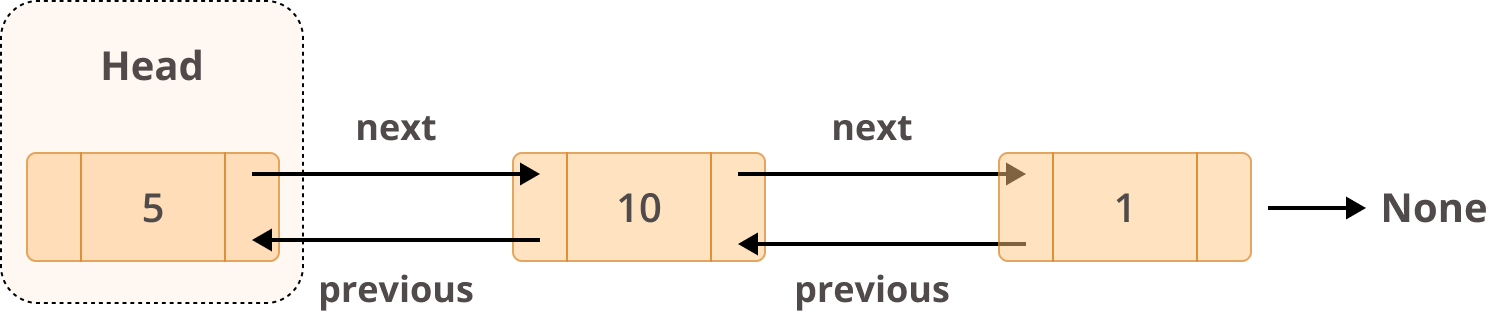
Doubly linked lists are different from singly linked lists in that they have two references:

  1. The previous field references the previous node.
  2. The next field references the next node.

The end result looks like this:

Example Node of a Doubly Linked ListNode (Doubly Linked List)

If you wanted to implement the above, then you could make some changes to your existing Node class in order to include a previous field:

class Node:
    def __init__(self, data):
        self.data = data
        self.next = None
        self.previous = None

This kind of implementation would allow you to traverse a list in both directions instead of only traversing using next. You could use next to go forward and previous to go backward.

In terms of structure, this is how a doubly linked list would look:

Example Structure of a Doubly Linked ListDoubly Linked List

You learned earlier that collections.deque uses a linked list as part of its data structure. This is the kind of linked list it uses. With doubly linked lists, deque is capable of inserting or deleting elements from both ends of a queue with constant O(1) performance.

How to Use Circular Linked Lists

Circular linked lists are a type of linked list in which the last node points back to the head of the list instead of pointing to None. This is what makes them circular. Circular linked lists have quite a few interesting use cases:

  • Going around each player’s turn in a multiplayer game
  • Managing the application life cycle of a given operating system
  • Implementing a Fibonacci heap

This is what a circular linked list looks like:

Example Structure of a Circular Linked ListCircular Linked List

One of the advantages of circular linked lists is that you can traverse the whole list starting at any node. Since the last node points to the head of the list, you need to make sure that you stop traversing when you reach the starting point. Otherwise, you’ll end up in an infinite loop.

In terms of implementation, circular linked lists are very similar to singly linked list. The only difference is that you can define the starting point when you traverse the list:

class CircularLinkedList:
    def __init__(self):
        self.head = None

    def traverse(self, starting_point=None):
        if starting_point is None:
            starting_point = self.head
        node = starting_point
        while node is not None and (node.next != starting_point):
            yield node
            node = node.next
        yield node

    def print_list(self, starting_point=None):
        nodes = []
        for node in self.traverse(starting_point):
            nodes.append(str(node))
        print(" -> ".join(nodes))

Traversing the list now receives an additional argument, starting_point, that is used to define the start and (because the list is circular) the end of the iteration process. Apart from that, much of the code is the same as what we had in our LinkedList class.

To wrap up with a final example, have a look at how this new type of list behaves when you give it some data:

>>>
>>> circular_llist = CircularLinkedList()
>>> circular_llist.print_list()
None

>>> a = Node("a")
>>> b = Node("b")
>>> c = Node("c")
>>> d = Node("d")
>>> a.next = b
>>> b.next = c
>>> c.next = d
>>> d.next = a
>>> circular_llist.head = a
>>> circular_llist.print_list()
a -> b -> c -> d

>>> circular_llist.print_list(b)
b -> c -> d -> a

>>> circular_llist.print_list(d)
d -> a -> b -> c

There you have it! You’ll notice that you no longer have the None while traversing the list. That’s because there is no specific end to a circular list. You can also see that choosing different starting nodes will render slightly different representations of the same list.

Conclusion

In this article, you learned quite a few things! The most important are:

  • What linked lists are and when you should use them
  • How to use collections.deque to implement queues and stacks
  • How to implement your own linked list and node classes, plus relevant methods
  • What the other types of linked lists are and what they can be used for

If you want to learn more about linked lists, then check out Vaidehi Joshi’s Medium post for a nice visual explanation. If you’re interested in a more in-depth guide, then the Wikipedia article is quite thorough. Finally, if you’re curious about the reasoning behind the current implementation of collections.deque, then check out Raymond Hettinger’s thread.

You can download the source code used throughout this tutorial by clicking on the following link:

Get the Source Code: Click here to get the source code you'll use to learn about linked lists in this tutorial.

Feel free to leave any questions or comments below. Happy Pythoning!


[ Improve Your Python With 🐍 Python Tricks 💌 – Get a short & sweet Python Trick delivered to your inbox every couple of days. >> Click here to learn more and see examples ]


from Planet Python
via read more

What Is The Machine Learning Engineer Salary?

According to the O’Reilly study The State of Machine Learning Adoption in the Enterprise, 50% of their respondents claim to have adopted machine learning to a different extent.  The demand for machine learning engineers is growing with the development of technology and new discoveries in the world of data science. More and more organizations decide […]

The post What Is The Machine Learning Engineer Salary? appeared first on neptune.ai.


from Planet SciPy
read more

TestDriven.io: Working with Static and Media Files in Django

This article looks at how to work with static and media files in a Django project, locally and in production. from Planet Python via read...